Band-limited waveform generation in Python/SciPy

readme.md

Returns periodic band-limited square, triangle, or sawtooth waveform with period 2π

Meant to be called the same way as scipy.signal.waveforms.square, but without the aliasing effects produced by the existing "naïve" implementation. Main goal is numerical accuracy for doing simulations, so the wave is generated by additive synthesis.

At low frequencies, the difference from the naive version is minimal, and the computational cost of the additive synthesis is high.

At high frequencies, the difference is very obvious, and the computational cost of additive synthesis is not too bad.

It currently requires a constant sampling frequency (no chirps) and doesn't support width or duty cycle.

Usage:

t = linspace(0, 1, num = 1000, endpoint = False)
plot(bl_square(2 * pi * 3 * t))

Waveform:

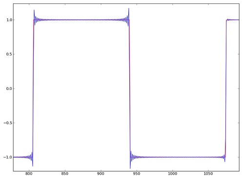
Band-limited version in blue, naïve version in red (equivalent to sampling the ideal mathematical function without putting it through an antialiasing filter first)

Spectra:

The extra spikes are the aliased harmonics, which are even more obvious when log-scaled:

dB-scaled spectra:

Sound examples:

• https://soundcloud.com/endolith/duty-cycle-sweep-aliased-vs-bandlimited-1
• https://soundcloud.com/endolith/weierstrass-sin-a-099-b-2

TODO:

Something like BLEPs might be better for this? (Probably not; they are not as accurate due to truncation of the sinc.)

Or the discrete summation methods would be more precise? Perhaps, but they cannot generate sawtooth/triangle/square directly, because the harmonic fall-off is at a different rate. They can generate BLITs, which can then be integrated to form the others, but this accumulates numerical error and requires leaky integration. Not sure how accurate that is.

With sweeps or chirps, there is also the problem of harmonics just disappearing suddenly when they hit fs/2 and producing sudden amplitude changes, which can be fixed with a roll-off filter, but which roll-off filter? It should probably be a parameter? But how to specify it as a parameter? I could also just cut it off suddenly, and let the user do their own filter, or oversample and decimate, if they want to. That's probably best.

No, you can't cut off the sweep frequencies so that one sample has a frequency and the next does not and then filter after the fact. The transition will cause a glitch with infinite harmonics that will alias, and post-filtering won't help. So it needs some kind of filter= argument for specifying the roll-off filter. Would it specify a filter object? and then harmonics are scaled by its frequency response? And filter=None should be possible which represents a brickwall! Then it will click for sweeps or go right up to Nyquist for non-sweeps if that's what's desired.

Also should have a phase={'zero', 'minimum', 'filter'} option.

bl_waveforms.py

# -*- coding: utf-8 -*-
"""
Bandlimited versions of scipy.signal.waveforms.

Intent is mathematical perfection over performance;
these use additive synthesis, so they are slow, but exact.

Less ideal methods using BLIT:
Sawtooth can be made by integrating BLIT minus a DC value to prevent integrator wandering off
Square can be made by integrating bipolar BLIT
Triangle can be made by integrating square
But I'm trying to avoid leaky integration, etc.
"""

from __future__ import division
from numpy import asarray, zeros, pi, sin, cos, amax, diff, arange, outer

# TODO: De-duplicate all this code into one generator function and then make these into wrapper functions

def bl_sawtooth(t): # , width=1
    """
    Return a periodic band-limited sawtooth wave with
    period 2*pi which is falling from 0 to 2*pi and rising at
    2*pi (opposite phase relative to a sin)

    Produces the same phase and amplitude as scipy.signal.sawtooth.

    Examples
    --------
    >>> t = linspace(0, 1, num = 1000, endpoint = False)
    >>> f = 5 # Hz
    >>> plot(bl_sawtooth(2 * pi * f * t))
    """
    t = asarray(t)

    if abs((t[-1]-t[-2]) - (t[1]-t[0])) > .0000001:
        raise ValueError("Sampling frequency must be constant")

    if t.dtype.char in ['fFdD']:
        ytype = t.dtype.char
    else:
        ytype = 'd'
    y = zeros(t.shape, ytype)

    # Get sampling frequency from timebase
    fs =  1 / (t[1] - t[0])
    #    fs =  1 / amax(diff(t))

    # Sum all multiple sine waves up to the Nyquist frequency

    # TODO: Maybe choose between these based on number of harmonics?

    # Slower, uses less memory
    for h in range(1, int(fs*pi)+1):
        y += 2 / pi * -sin(h * t) / h

    # Faster, but runs out of memory and dies
#    h = arange(1, int(fs * pi) + 1)
#    phase = outer(t, h)
#    y = 2 / pi * -sin(phase) / h
#    y = sum(y, axis=1)

    return y


def bl_triangle(t):
    """
    Return a periodic band-limited triangle wave with
    period 2*pi which is falling from 0 to pi and rising from
    pi to 2*pi (same phase as a cos)

    Produces the same phase and amplitude as scipy.signal.sawtooth(width=0.5).

    Examples
    --------
    >>> t = linspace(0, 1, num = 1000, endpoint = False)
    >>> f = 5 # Hz
    >>> plot(bl_triangle(2 * pi * f * t))
    """
    t = asarray(t)

    if abs((t[-1]-t[-2]) - (t[1]-t[0])) > .0000001:
        raise ValueError("Sampling frequency must be constant")

    if t.dtype.char in ['fFdD']:
        ytype = t.dtype.char
    else:
        ytype = 'd'
    y = zeros(t.shape, ytype)

    # Get sampling frequency from timebase
    fs =  1 / (t[1] - t[0])

    # Sum all odd multiple sine waves up to the Nyquist frequency

    # Slower, uses less memory
    for h in range(1, int(fs * pi) + 1, 2):
        y += 8 / pi**2 * -cos(h * t) / h**2

    # Faster, but runs out of memory and dies
#    h = arange(1, int(fs * pi) + 1, 2)
#    phase = outer(t, h)
#    y = 8 / pi**2 * -cos(phase) / h**2
#    y = sum(y, axis=1)

    return y


def bl_square(t, duty=0.5):
    """
    Return a periodic band-limited square wave with
    period 2*pi which is +1 from 0 to pi and -1 from
    pi to 2*pi (same phase as a sin)

    Produces the same phase and amplitude as scipy.signal.square.

    Similarly, duty cycle can be set, or varied over time.

    Examples
    --------
    >>> t = linspace(0, 1, num = 10000, endpoint = False)
    >>> f = 5 # Hz
    >>> plot(bl_square(2 * pi * f * t))

    >>> sig = np.sin(2 * np.pi * t)
    >>> pwm = bl_square(2 * np.pi * 30 * t, duty=(sig + 1)/2)
    >>> plt.subplot(2, 1, 1)
    >>> plt.plot(t, sig)
    >>> plt.subplot(2, 1, 2)
    >>> plt.plot(t, pwm)
    >>> plt.ylim(-1.5, 1.5)
    """
    return bl_sawtooth(t - duty*2*pi) - bl_sawtooth(t) + 2*duty-1


def blit(t):
    """
    Return a periodic band-limited impulse train (Dirac comb) with
    period 2*pi (same phase as a cos)

    Examples
    --------
    >>> t = linspace(0, 1, num = 1000, endpoint = False)
    >>> f = 5.4321 # Hz
    >>> plot(blit(2 * pi * f * t))

    References
    ----------
    http://www.music.mcgill.ca/~gary/307/week5/bandlimited.html
    """
    t = asarray(t)

    if abs((t[-1]-t[-2]) - (t[1]-t[0])) > .0000001:
        raise ValueError("Sampling frequency must be constant")

    if t.dtype.char in ['fFdD']:
        ytype = t.dtype.char
    else:
        ytype = 'd'
    y = zeros(t.shape, ytype)

    # Get sampling frequency from timebase
    fs =  1 / (t[1] - t[0])

    # Sum all multiple sine waves up to the Nyquist frequency
    N = int(fs * pi) + 1
    for h in range(1, N):
        y += cos(h * t)
    y /= N

#    h = arange(1, int(fs * pi) + 1)
#    phase = outer(t, h)
#    y = 2 / pi * cos(phase)
#    y = sum(y, axis=1)

    return y


if __name__ == "__main__":
    from numpy import linspace
    import matplotlib.pyplot as plt
    from scipy.signal import square, sawtooth

    fs = 500
    t = linspace(0, 1, num = fs, endpoint = False)
    f = 5.432 # Hz

    # Test that waveforms match SciPy versions
    plt.figure()
    plt.subplot(3, 1, 1)
    plt.plot(t,    square(2 * pi * f * t), color='gray')
    plt.plot(t, bl_square(2 * pi * f * t))
    plt.title('Square')

    plt.subplot(3, 1, 2)
    plt.plot(t,    sawtooth(2 * pi * f * t, 0.5), color='gray')
    plt.plot(t, bl_triangle(2 * pi * f * t))
    plt.title('Triangle')

    plt.subplot(3, 1, 3)
    plt.plot(t,    sawtooth(2 * pi * f * t), color='gray')
    plt.plot(t, bl_sawtooth(2 * pi * f * t))
    plt.title('Sawtooth')


    # Square wave duty cycle test
    plt.figure()
    plt.subplot(3, 1, 1)
    width = 0.5
    plt.plot(t,    square(2*pi*f*t, width), color='gray')
    plt.plot(t, bl_square(2*pi*f*t, width))
    plt.margins(0, 0.1)

    plt.subplot(3, 1, 2)
    width = 0.01
    plt.plot(t,    square(2*pi*f*t, width), color='gray')
    plt.plot(t, bl_square(2*pi*f*t, width))
    plt.margins(0, 0.1)

    plt.subplot(3, 1, 3)
    width = 2/3
    plt.plot(t,    square(2*pi*f*t, width), color='gray')
    plt.plot(t, bl_square(2*pi*f*t, width))
    plt.margins(0, 0.1)

Hi,
Thanks for sharing this Gist. I'm pretty new to the topic, but do you have any advice on how to create the additive version of the Spectra image you upload with Additive Synthesis?

Thanks,

@wdputro I don't understand the question. This is additive synthesis.

scipy/scipy#1507