Skip to content

Instantly share code, notes, and snippets.

@jessvb
Last active January 27, 2024 15:21
Show Gist options
  • Star 5 You must be signed in to star a gist
  • Fork 3 You must be signed in to fork a gist
  • Save jessvb/4d074469e7533530df758aa482ae3d07 to your computer and use it in GitHub Desktop.
Save jessvb/4d074469e7533530df758aa482ae3d07 to your computer and use it in GitHub Desktop.
Notes for how to approach and do certain statistical tests. The particular details are in Python, but a lot of the notes are generalizable.

How to approach statistics

Before you code, do three things:

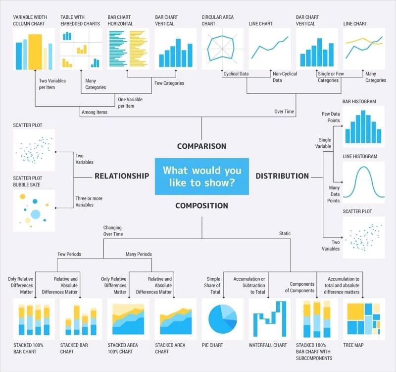
  1. Think about what you want to show in your data. For example, how would you like to ultimately visualize it or what would you ultimately like to say about it? Here are some helpful info graphics from a data science cheatsheet article on Medium:

image

image

  1. Do quick initial visualizations of your data to get a sense of their distributions, whether it's actually worth doing a statistical test (i.e., does it look like there might be a significant difference?), and whether there are any outliers (which could be interesting in themselves! E.g., why did that particular participant choose xyz vs. how the rest of the group chose?). Diverging stacked bar charts are excellent as first visualizations for ordinal data (like Likert Scale data), and box plots are also excelent first visualizations for other data. JMP is apparently great for these types of initial quick-looks, and Vega-Lite (e.g., Vega-Lite editor, normalized stacked bar chart) is awesome for creating visualizations right in the browser with JSON (e.g., use csv to json converter or python pandas to_json) or with Python/Jupyter.

    1. With these plots, you'll get a sense of:
      1. the distribution (e.g., if it's skewed to the left or right, it might not be normal),
      2. see whether the two distributions you're comparing are similar (and if not, figure out if there are different subgroups of the data that are causing different distributions),
      3. see if there are outliers (and why this might be the case → Is there a particular type of person/variable that's causing the outliers?), and
      4. figure out if it's worth it to do a statistical test (e.g., if the distributions are similar, but the medians are different).
    2. Here are some useful links about how to analyze box plots:
      1. Interpreting box plots by Khan Academy (e.g., T/F statements about box plots)
      2. How to compare box plots by Linh Ngo
      3. More on how to compare box plots by Linh Ngo
    3. See this paper about why diverging stacked bar charts are ideal for visualizing Likert scale results.
      1. Robbins, Naomi B., and Richard M. Heiberger. "Plotting Likert and other rating scales." Proceedings of the 2011 joint statistical meeting. Vol. 1. American Statistical Association,, 2011.
  2. Figure out which type of statistical test you need to use; for example, by using the flowchart below from this article. image

    1. The first question to ask yourself is: Is your data normal? In many of the code snippets below, this question is taken care of for you by a normality test, and the appropriate test will automatically be chosen (e.g., if normal --> t-test).

      1. Note also that if you have a sample size n > 30, "according to the central limit theorem, the distribution of the sample mean satisfies the normal distribution when the number of samples is above 30", so you do not necessarily have to check for normality [Normality Test in Clinical Research, Central limit theorem: the cornerstone of modern statistics].
    2. The second question is: Is your data paired or unpaired? Paired data is usually where you follow individuals through the data, like when you're trying to find differences between pre/post surveys. Unpaired data is where you're finding differences between different "groups" of participants, like parents vs. children on a specific survey. For paired data, you use tests like the "paired t-test" (normal) and the "Wilcoxon signed-rank test" (not normal). For unpaired data, you use tests like the "independent t-test" (normal) and the "Mann-Whitney U test" (not normal).

    3. Other tests might include Kendall Tau correlation, Krippendorff's alpha for computing inter-coder reliability for thematic analysis, etc.

More complex statistics: When you have many comparisons, factors, covariates, etc.

If you're considering doing a lot of comparisons because you have a large number of factors/covariates that could potentially affect your dependent variable, don't do it! Doing many comparisons (e.g., with a t-test) increases the chances of incorrect results. Use ANOVA/ANCOVA/MANCOVA/regression/etc. instead! Quote from "Biofeedback Heart Rate Training during Exercise" by Goldstein et al.:

The experimental data were analyzed in two steps. First, analyses of
variance (ANOVAs) were performed and then independent means t-tests
comparing the experimental groups. The reason for this apprach was that
the data analysis involved multiple between-group comparisons, and the
probability that at least one of these would reveal a statistically significant
difference by chance alone was unacceptably high. ANOVAs provided an
assessment of the significance of the overall effects of feedback, sessions,
etc., on the dependent variables, and obtaining significant effects in the
ANOVAs permitted application of multiple t-tests to the data without fear
of wrongly inferring significant differences between groups.

Here's a link to a fantastic explanation of the differences between ANOVA, ANCOVA, MANOVA, & MANCOVA. Below, pictures from the site explain the differences in a nutshell.

Side Note:

  • "Dependent Variable" == output (e.g., someone's heart rate)
  • "Independent Variables" == input variables that don't change (e.g., users' age or the app version), which can be either "factors" or "covariates"
  • "Covariates" == continuous independent variable (e.g., age, number of hours spent studying, or anxiety-trait score)
  • "Factor" == independent variable that comes in "groups" and is not continuous (e.g., gender, level of education, or app version)

Side Note:

ANOVA, ANCOVA, linear regression, etc. methods expect the output ("dependent") variable to be continuous. If you have oridinal data, like Likert scale data, technically you're supposed to use ordinal methods instead, like ordered logistic regression, multinomial logistic regression, or binary logistic regression [Analysing Likert Scale Type Data]. That being said, you can treat Likert scale data as continuous if either:

ANOVA

One-Way ANOVA Two-Way ANOVA
image image
  • Input: one or two factors (i.e., with levels/groups)
  • Output: one continuous variable

ANCOVA

image (Basically ANOVA, but also includes at least one covariate / continuous independent variable.)

  • Input: factors and covariates
  • Output: one continuous variable

How to implement ANCOVA

Here are some links describing ANCOVA and Linear Regression [ANCOVA expressed as linear regression, How to perform ANCOA in Python, How to fit models using formulas & categorical variables]. Essentially, you can use the statsmodels.api package, statsmodels.formula.api package, and the ols function to model your data (Linear Regression), and get summary statistics. Use the p-values in the summary to determine if they likely affect the outcome of the dependent variable.

Make sure to test the assumptions for linear regression though! See this post on how to test linear regression assumptions in Python.

Here's a code snippet of how to model data with both categorical (C()) and covariate independent variables.

import pandas as pd
import statsmodels.api as sm
import statsmodels.formula.api as smf

# Example dataframe:
df = pd.read_csv("avg-hr-by-app-type.csv")
df.head()
avgHR appType expLevel gender anxietyTrait age busyness
57.956522 A advanced male 1.6 19 0.5025
88.900000 B novice female 1.6 31 0.4775
100.388889 A advanced male 2.0 42 0.4775
105.981132 B novice female 1.4 22 0.3450
82.645161 A advanced male 1.0 39 0.3600
# ANCOVA (Note: C --> categorical variable)
formula = "avgHR ~ C(appType) + C(expLevel) + C(gender) + anxietyTrait + age + busyness"
model = smf.ols(formula=formula, data=df).fit()
model.summary()

At the top of the model summary, find the R-squared and the Prob (F-statistic) values. These tell you the goodness-of-fit. See Regression Analysis by Example by Chatterjee & Hadi for in-depth discussion of linear regression.

E.g., "The goodness-of-fit index, R^2, may be interpreted as the proportion [percent] of the total variability in the response variable Y that is accounted for by the predictor variable[s]"

E.g., "H_0 is rejected if ... p(F) <= alpha", and "H_0: Reduced model is adequate ... H_1: Full model is adequate" (i.e., if p < alpha, the full model/formula you developed is likely significant!)

If you can't satisfy the linearity assumption or can't come up with a model where p < alpha, R^2 is great enough, etc., consider adding more variables to your formula and/or interaction effects, or transforming the dependent variable (e.g., log(y)). Here's some more info on transformations:

MANOVA

One-Way MANOVA Two-Way MANOVA
image image

(Basically ANOVA, but has multiple output/dependent variables.)

  • Input: one or two factors
  • Output: multiple continuous variables

MANCOVA

image (Basically ANCOVA, but has multiple output/dependent variables.)

  • Input: factors and covariates
  • Output: multiple continuous variables

Stats in Python

See the following code snippets for how to do stats in Python:

More detail about methods used above:

import pandas as pd
###############################################################################
### Prepare data for paired statistical tests.
### For paired tests, you need to keep track of IDs of the participants and
### compare them across surveys. This shows an example where there was a pre-,
### mid-, and post-survey, and the IDs are stored in a column named "codename".
def onlySameIds(data1, data2, idname='codename'):
data1_for_data2 = data1.loc[data1[idname].isin(
data2[idname])].sort_values(by=[idname])
data2_for_data1 = data2.loc[data2[idname].isin(
data1[idname])].sort_values(by=[idname])
return (data1_for_data2, data2_for_data1)
predata = pd.read_excel('path/to/pre-survey.xlsx', sheet_name="cleaned-responses")
middata = pd.read_excel('path/to/mid-survey.xlsx', sheet_name="cleaned-responses")
postdata = pd.read_excel('path/to/post-survey.xlsx', sheet_name="cleaned-responses")
# get the independent columns either by listing them, like this, or from the
# data itself (e.g., you could use the df.columns attribute somehow...)
indep_cols = [
"levelprogramming",
"childparent",
"age",
"gender"
]
# Assuming that you just collected the demographics/independent variable information
# in the pre-survey, you'll have to add the independent variable columns from pre-survey
# to middata and postdata:
# 1. find unique indep_cols
cols_to_add = []
for col in indep_cols:
if not col in middata.columns: # here, we could put postdata or middata - doesn't matter
cols_to_add.append(col)
cols_to_add.append("codename") # include codename column for merging
data_to_add = predata[cols_to_add]
# 2. add the columns to middata and postdata, only keeping rows from 'left'
# dataframes, which are middata and postdata (not data_to_add) in this case
# (note: merge "defaults to the intersection of the columns in both
# DataFrames", which in this case will be "codename". You can alternatively
# manually input which column(s) it will be merged on.)
middata = middata.merge(data_to_add, how='left')
postdata = postdata.merge(data_to_add, how='left')
# Next, let's make sure to clean the data s.t. we're comparing the same/correct students pre
# vs. post vs. mid. Only look at IDs that are in BOTH pre and mid data:
(predata_for_mid, middata_for_pre) = onlySameIds(predata, middata, 'codename')
(predata_for_post, postdata_for_pre) = onlySameIds(predata, postdata, 'codename')
(middata_for_post, postdata_for_mid) = onlySameIds(middata, postdata, 'codename')
# The data should be good to go now! See 2-paired-t-test-and-wilx-helper-functions.py for the
# actual comparisons.
################################################################################
#################################################################################
### Helper functions for normality, paired t-test and wilcoxon tests
# See first 01-paired-data-prep.py
# You may want to loop over the following functions for large datasets and create
# a dataframe and/or an Excel spreadsheet of the data. (See below.)
###############################
########## functions ##########
# This will perform a t-test or wilcoxon signed-rank test depending on a normality
# test of the differences between two columns (e.g., pre/post) and print out the
# results.
# e.g., data1 = pre-test with many columns of likert scale values
# e.g., data2 = post-test with many columns of likert scale values
# e.g., comparisonName = 'pre/post' --> this is just to print
# e.g., col = 'likertQ1' --> this is the column name in data1/data2 you're comparing
def compareData(data1, data2, col, comparisonName, alpha=0.05):
# to add to dataframe: depencol | indepcol[s] | datapair[2] | greater/less | testname | pval | stat | init_mean | after_mean
# actual col names: depen | indep | comparison | sigdir | test | p | stat | mean1 | mean2
# e.g., friendcoworker | numagents=3 | pre/post | -1 | wilx | pval | stat | 2.2 | 1.5
datatoappend = None
diffs = getDiffs(data1, data2, col)
if colsAreComparable(data1, data2, col):
testname = 'n/a'
res = {'pvalue': None, 'statistic': None, 'z_abs': None}
if (sum(diffs) != 0):
if isNormal(data1, data2, col, alpha):
# paired t-test
restest = stats.ttest_rel(data1[col], data2[col])
testname = 'ttest'
else:
# wilcoxon signed-rank test
restest = stats.wilcoxon(diffs)
testname = 'wilx'
mean1 = data1[col].mean()
mean2 = data2[col].mean()
if (sum(diffs) != 0) and (restest.pvalue < alpha):
res['pvalue'] = restest[1]
res['statistic'] = restest[0]
greaterless = 0
if mean1 > mean2:
greaterless = -1
elif mean1 < mean2:
greaterless = 1
# summarize data in a dictionary to be added to a dataframe/spreadsheet:
datatoappend = {'depen': col, 'indep1': None, 'indep2': None, 'indep3': None,
'comparison': comparisonName, 'sigdir': greaterless,
'testname': testname, 'p': res['pvalue'], 'stat': res['statistic'],
'mean1': mean1, 'mean2': mean2} # still need: indep
else:
print(
f'not significant ({col}: {comparisonName}; mean1: {mean1}, mean2: {mean2})')
else:
print('NOTE: columns are *not* comparable')
print(
f'comparison: {col}: {comparisonName}; len data 1: {len(data1)}; len data 2: {len(data2)}')
return datatoappend
def colsAreComparable(data1, data2, colname):
comparable = False
if (colname in data1) and (colname in data2):
if (len(data1) > 0) and (len(data2) > 0):
if is_numeric_dtype(data1[colname]) and is_numeric_dtype(data2[colname]):
comparable = True
else:
print('not comparable because len <= 0')
else:
print('not comparable because colname not in one of datas')
print(f'colname: {colname}')
return comparable
def isNormal(data1, data2, colname, alpha=0.05):
normal = True
if (len(data1[colname]) < 20 or len(data2[colname]) < 20):
normal = False
else:
res1 = stats.normaltest(data1[colname])
res2 = stats.normaltest(data2[colname])
if (res1.pvalue < alpha) or (res2.pvalue < alpha):
normal = False
return normal
def getDiffs(data1, data2, colname):
diffs = []
for id in data1['codename'].values:
diff = data2.loc[data2['codename'] == id][colname].values[0] - \
data1.loc[data1['codename'] == id][colname].values[0]
# check if NaN (could have a missing value) and add to diffs:
if not math.isnan(diff):
diffs.append(float(diff))
return diffs
###################################
########## Example usage ##########
# See 1-paired-data-prep.py to get and prepare data.
alpha = 0.05
# ...
### Single comparison example ###
nameinit = 'pre'
namefin = 'mid'
depencol = 'unreliabledependable'
limcol1 = 'weird'
lim1 = 0
limcol2 = None
lim2 = None
if nameinit == 'pre' and namefin == 'mid':
datainit = predata_for_mid
datafin = middata_for_pre
elif nameinit == 'pre' and namefin == 'post':
datainit = predata_for_post
datafin = postdata_for_pre
elif nameinit == 'mid' and namefin == 'post':
datainit = middata_for_post
datafin = postdata_for_mid
else:
print("INCORRECT NAMES FOR DATA")
if (limcol2):
data1 = datainit.loc[(datainit[limcol1] == lim1) &
(datainit[limcol2] == lim2)]
data2 = datafin.loc[(datafin[limcol1] == lim1) &
(datafin[limcol2] == lim2)]
datatoappend = compareData(
data1, data2, depencol, f'{nameinit}/{namefin}', alpha)
datatoappend['indep1'] = f'{limcol1}={lim1}'
datatoappend['indep2'] = f'{limcol2}={lim2}'
else:
data1 = datainit.loc[(datainit[limcol1] == lim1)]
data2 = datafin.loc[(datafin[limcol1] == lim1)]
datatoappend = compareData(
data1, data2, depencol, f'{nameinit}/{namefin}', alpha)
datatoappend['indep1'] = f'{limcol1}={lim1}'
# PRINT
print(datatoappend)
### Loop over many examples ###
depen_cols = ["likertQ1", "likertQ2", "likertQ3", "..."]
datapairs = [
[predata_for_mid, middata_for_pre, 'pre/mid'],
[predata_for_post, postdata_for_pre, 'pre/post'],
[middata_for_post, postdata_for_mid, 'mid/post']
]
resdf = pd.DataFrame(columns=['depen', 'indep1', 'indep2', 'indep3', 'comparison',
'sigdir', 'testname', 'p', 'stat', 'mean1', 'mean2'])
for datapair in datapairs:
for depencol in depen_cols:
datatoappend = compareData(datapair[0], datapair[1], depencol, datapair[2], alpha)
resdf = resdf.append(datatoappend, ignore_index=True)
# export the data to an excel spreadsheet
filename = 'paired-results.xlsx'
resdf.to_excel(filename)
print(f"--- Exported to spreadsheet: {filename} ---")
import pandas as pd
###############################################################################
### Prepare data for paired statistical tests.
### For unpaired tests, you *don't* to keep track of IDs of the participants,
### so it's a little simpler than for paired prep.
predata = pd.read_excel('path/to/pre-survey.xlsx', sheet_name="cleaned-responses")
middata = pd.read_excel('path/to/mid-survey.xlsx', sheet_name="cleaned-responses")
postdata = pd.read_excel('path/to/post-survey.xlsx', sheet_name="cleaned-responses")
# get the independent columns either by listing them, like this, or from the
# data itself (e.g., you could use the df.columns attribute somehow...)
indep_cols = [
"levelprogramming",
"childparent",
"age",
"gender"
]
# Assuming that you just collected the demographics/independent variable information
# in the pre-survey, you'll have to add the independent variable columns from pre-survey
# to middata and postdata:
# 1. find unique indep_cols
cols_to_add = []
for col in indep_cols:
if not col in middata.columns: # here, we could put postdata or middata - doesn't matter
cols_to_add.append(col)
cols_to_add.append("codename") # include codename column for merging
data_to_add = predata[cols_to_add]
# 2. add the columns to middata and postdata, only keeping rows from 'left'
# dataframes, which are middata and postdata (not data_to_add) in this case
# (note: merge "defaults to the intersection of the columns in both
# DataFrames", which in this case will be "codename". You can alternatively
# manually input which column(s) it will be merged on.)
middata = middata.merge(data_to_add, how='left')
postdata = postdata.merge(data_to_add, how='left')
# The data should be good to go now! See 4-unpaired-t-test-and-mann-whitney-helper-functions.py for the
# actual comparisons.
##################################################################################
# Mann-Whitney Test
# See first, 03-unpaired-data-prep.py.
# Assumption: Data are independent (e.g., Likert scale from parents vs. children.
#
# See example: https://docs.scipy.org/doc/scipy/reference/generated/scipy.stats.mannwhitneyu.html
#
# If the differences between the two samples *are* normally distributed, use an
# independent t-test: scipy.stats.ttest_ind
# https://docs.scipy.org/doc/scipy/reference/generated/scipy.stats.ttest_ind.html#scipy.stats.ttest_ind
alpha = 0.05
# ... see 03-unpaired-data-prep.py ...
#################
### functions ###
def isNormal(data1, data2, colname, alpha=0.05):
normal = True
if (len(data1[colname]) < 20 or len(data2[colname]) < 20):
normal = False
else:
res1 = stats.normaltest(data1[colname])
res2 = stats.normaltest(data2[colname])
if (res1.pvalue < alpha) or (res2.pvalue < alpha):
normal = False
return normal
def colsAreComparable(data1, data2, colname):
comparable = False
if (colname in data1) and (colname in data2):
if (len(data1) > 0) and (len(data2) > 0):
if is_numeric_dtype(data1[colname]) and is_numeric_dtype(data2[colname]):
comparable = True
else:
print('not comparable because len <= 0')
else:
print('not comparable because colname not in one of datas')
print(f'colname: {colname}')
return comparable
def compareData(data1, data2, col, comparisonName, alpha=0.05):
# to add to dataframe: demographics | comparisonname | pre or mid or post | indepcol[s] | greater/less | testname | pval | stat | init_mean | after_mean
# actual col names: demog | comparison | whichdata | indep1 | indep2 | indep3 | sigdir | test | p | stat | mean1 | mean2
# e.g., levelprogramming | weird-0v1 | predata | children | None | None | -1 | wilx | pval | stat | 2.2 | 1.5
datatoappend = None
if colsAreComparable(data1, data2, col):
testname = 'n/a'
res = {'pvalue': None, 'statistic': None, 'z_abs': None}
if isNormal(data1, data2, col, alpha):
# independent t-test
restest = stats.ttest_ind(data1[col], data2[col])
testname = 'ttest'
else:
# mann-whitney test
restest = stats.mannwhitneyu(data1[col], data2[col])
testname = 'mann-whitney'
mean1 = data1[col].mean()
mean2 = data2[col].mean()
if restest.pvalue < alpha:
res['pvalue'] = restest[1]
res['statistic'] = restest[0]
greaterless = 0
if mean1 > mean2:
greaterless = -1
elif mean1 < mean2:
greaterless = 1
# summarize data in a dictionary to be added to a dataframe/spreadsheet:
datatoappend = {'demog': col, 'comparison': comparisonName, 'whichdata': None,
'indep1': None, 'indep2': None, 'indep3': None, 'sigdir': greaterless,
'test': testname, 'p': res['pvalue'], 'stat': res['statistic'],
'mean1': mean1, 'mean2': mean2} # still need: comparison(actual), indep[s], whichdata
else:
print(
f'not significant ({col}: {comparisonName}; mean1: {mean1}, mean2: {mean2})')
else:
print('NOTE: columns are *not* comparable')
print(
f'comparison: {col}: {comparisonName}; len data 1: {len(data1)}; len data 2: {len(data2)}')
return datatoappend
###########################
### Example comparisons ###
##### Single comparison #####
### REGULAR ###
data = predata
whichdata = 'predata'
depencol = 'unreliabledependable'
compcol = 'weird'
comp1 = 0
comp2 = 1
limcol = None # 'weird'
limit = None # 0
if (limcol):
data1 = data.loc[(data[compcol] == comp1) &
(data[limcol] == limit)]
data2 = data.loc[(data[compcol] == comp2) &
(data[limcol] == limit)]
datatoappend = compareData(
data1, data2, depencol, f'{limcol}={limit} {compcol}-{comp1}v{comp2}', alpha)
else:
data1 = data.loc[(data[compcol] == comp1)]
data2 = data.loc[(data[compcol] == comp2)]
datatoappend = compareData(
data1, data2, depencol, f'{compcol}-{comp1}v{comp2}', alpha)
# ### GREATER THAN / LESS THAN ETC. WITH LIM ###
# data = predata
# whichdata = 'predata'
# depencol = 'inflexibleflexible'
# compcol = 'numagents'
# comp1 = 1
# comp2 = 1
# limcol = 'weird'
# limit = 0
# data1 = data.loc[(data[compcol] == comp1) &
# (data[limcol] == limit)]
# data2 = data.loc[(data[compcol] > comp2) &
# (data[limcol] == limit)]
# datatoappend = compareData(data1, data2, depencol, f'{limcol}={limit} {compcol}-=={comp1}v>{comp2}', alpha)
# ### GREATER THAN / LESS THAN ETC. NO LIM ###
# data = predata
# whichdata = 'predata'
# depencol = 'trustcas'
# compcol = 'numagents'
# comp1 = 1
# comp2 = 1
# limcol = None
# limit = None
# data1 = data.loc[(data[compcol] == comp1)]
# data2 = data.loc[(data[compcol] > comp2)]
# datatoappend = compareData(data1, data2, depencol, f'{compcol}-=={comp1}v>{comp2}', alpha)
### PRINT ###
if(datatoappend):
datatoappend['whichdata'] = whichdata
if limcol:
datatoappend['indep1'] = limcol
print(datatoappend)
##### Loop over many examples #####
depen_cols = ["likertQ1", "likertQ2", "likertQ3", "..."]
resdf = pd.DataFrame(columns=['depen', 'comparison', 'whichdata', 'indep1',
'indep2', 'indep3', 'sigdir', 'test', 'p', 'stat', 'mean1', 'mean2'])
for data, dataname in zip(alldata, datanames): # e.g., within predata
for indepcol in indep_cols: # e.g., levelprogramming
if (indepcol in data):
i = 0
categories = data[indepcol].unique() # e.g., levelprogramming -> 0, 1, 2, 3
# for categ in categories: # e.g., childparent='C' vs childparent='P'
while i < len(categories):
j = i + 1
# e.g., compare depen cols ('likertQ1', 'likertQ2') btwn parent vs child
while j < len(categories):
data1 = data.loc[data[indepcol] == categories[i]]
data2 = data.loc[data[indepcol] == categories[j]]
for depencol in depen_cols:
datatoappend = compareData(data1, data2, depencol, f'{indepcol}-{categories[i]}v{categories[j]}', alpha)
datatoappend['whichdata'] = dataname
resdf = resdf.append(datatoappend, ignore_index=True)
j += 1
i += 1
# export the data to an excel spreadsheet
filename = 'unpaired-results.xlsx'
resdf.to_excel(filename)
print(f"--- Exported to spreadsheet: {filename} ---")
### Potential correlation tests:
# If Normal: Pearson correlation, but has to be interval or ratio data (NOT ordinal/categorical)
# If Not Normal --> non-parametric tests
# Non-parametric tests:
# (1) Spearman: for interval or ratio data (NOT ordinal/categorical)
# (2) Kendall: for ordinal or continuous data :)
# --> I think you can use Kendall for any of not-normal/normal/oridinal/continuous
### Test your data for normality. If some of the columns are not normal and/or some are ordinal,
### then use the Kendall correlation
# test normality (NOTE: you can't do this with string data):
# for s in cordata.columns:
# # print(cordata[s])
# k2, p = stats.normaltest(cordata[s])
# if p < alpha:
# print('normal: ' + str(s))
# else:
# print('NOT NORMAL: ' + str(s))
# # since some are not normal, let's use non-parametric test
import pandas as pd
import seaborn as sn
import matplotlib.pyplot as plt
import re
from scipy import stats
alpha = 0.05
predata = pd.read_excel('path/to/predata.xlsx')
postdata = pd.read_excel('path/to/postdata.xlsx')
otherdata = pd.read_excel('path/to/any/other/data.xlsx')
alldata = pd.merge(otherdata, pd.merge(predata,postdata, on='ID', suffixes=('_pre','_post')), on='ID')
# only columns we want to correlate:
cordata = pd.DataFrame(alldata,columns=[
'example_col_pre', 'example_col_post', 'example_col2_pre', 'example_col2_post', 'other_col'
])
# clean data (get rid of rows with NaN's):
cordata = cordata.dropna()
# get the correlation matrix
corrMatrix = cordata.corr(method='kendall')
sn.heatmap(corrMatrix, annot=True)
plt.tight_layout()
plt.savefig('./path/to/figstorage/correlation-matrix.png', dpi=400)
plt.show()
print(corrMatrix)
# test for strong correlations (abs(cor) > ~0.5) and med (abs(cor) > ~0.3)
# NOTE: it's a symmetric matrix, so let's just do the bottom triangle
strong = []
med = []
c = 0
for col in corrMatrix.columns:
c += 1 # skip the diagonal (which is always 1.0)
for r in range(c,len(corrMatrix)):
row = corrMatrix.columns[r]
if corrMatrix[col][r] >= 0.5:
# print('strong correlation: ' + str(col) + ' & ' + str(row))
coef, p = stats.kendalltau(cordata[col], cordata[row])
if p < alpha:
# print(' significant')
strong.append((col, row))
# else:
# print(' NOT significant')
# print()
elif corrMatrix[col][r] >= 0.3:
# print('med correlation: ' + str(col) + ' & ' + str(row))
coef, p = stats.kendalltau(cordata[col], cordata[row])
if p < alpha:
# print(' significant')
med.append((col, row))
# else:
# print(' NOT significant')
# print()
print('Strong Correlations:')
for t in strong:
print(str(t[0]) + ', ' + str(t[1]))
print()
print('Medium Correlations:')
for t in med:
print(str(t[0]) + ', ' + str(t[1]))
# NOTE: Interpretation of strong/med correlations:
# Values of 0.5 for strong and 0.3 for med come from education psychology:
# “Statistical Power Analysis for the Behavioral Sciences” 2013, pg. 80-81
# NOTE: Meaning of the p-value for strength:
# coef, p = scipy.stats.kendalltau(data1, data2)
# → This gives you the value in the matrix (coef) and the p-value → test whether the p-value is < 0.05
# From paper on User’s guide to correlation coefficients: https://www.ncbi.nlm.nih.gov/pmc/articles/PMC6107969/
# - p-value doesn’t mean the strength of the correlation, it means the likelihood that the correlation is actually this
# strength (whether that’s weak strength or strong)
# - e.g., “The low level of the p-value reassures us that 99.99% of the time the correlation is *weak* at an r of 0.31.”
################################################################################
### Use this for inter-coder reliability (ICR, IRR, interrater agreement, etc.)
### when performing thematic analysis / open coding on data where you have
### multiple coders, and can tag items with multiple codes: Krippendorff's
### Alpha with MASI distance.
###
### For more information about many different ICR methods, see, "Intercoder
### Reliability in Qualitative Research: Debates and Practical Guidelines" by
### O'Connor and Joffe.
###
### For a citable paper on this specific ICR method, see "Inter-Coder Agreement
### for Computational Linguistics" by Artstein and Poesio.
###
### This code was taken from dashtaisen on StackOverflow:
### https://stackoverflow.com/questions/45741934/low-alpha-for-nltk-agreement-using-masi-distance
import pandas as pd
import nltk
from nltk.metrics import agreement
from nltk.metrics.distance import masi_distance
from nltk.metrics.distance import jaccard_distance
### get data
# Assumes columns are sorted by content (i.e., items to be tagged) so that all
# of the same content is next to each other in the list, and that there are
# no nulls / empty rows until the very end of the columns. (You can use 10-25%
# of your full dataset https://journals.sagepub.com/doi/10.1177/1609406919899220)
# e.g., name1_tag name1_content name2_tag name2_content
# +Artificial cute robot +Artificial cute robot
# Approachable cute robot Personalized depends on topic
# Personalized depends on topic Convenient not smart
data = pd.read_excel('path/to/spreadsheet.xlsx', sheet_name="krippendorffs_alpha_prep")
### put data into correct format for krippendorff's: (coder, item, label)
def getkripdata(data, coders):
tagdata = []
for coder in coders:
i = 0
currTags = []
while i < len(data[f"{coder}_content"]) - 1:
currItem = data[f"{coder}_content"][i]
nextItem = data[f"{coder}_content"][i+1]
currTag = data[f"{coder}_tag"][i]
currTags.append(currTag)
if ((nextItem != currItem)):
if pd.notna(currItem):
tagdata.append((f"{coder}",currItem,frozenset(currTags)))
currTags = []
i += 1
# append the last tags/items
if data[f"{coder}_content"][i] == currItem:
currTags.append(data[f"{coder}_tag"][i])
else:
currItem = data[f"{coder}_content"][i]
currTags = [data[f"{coder}_tag"][i]]
if pd.notna(currItem):
tagdata.append((coder,currItem,frozenset(currTags)))
return tagdata
# In this case, we have 3 coders, where each coder overlapped with the other
# coders for a certain portion of the text. (Alternatively, you could just have
# 2 coders, so you'd just need `coders=[name1,name2]`.)
# e.g., name1forname2_tag name1forname2_content name2forname1_tag name2forname1_content name1forname3_tag name1forname3_content name3forname1_tag ...
# (vs. name1_tag name1_content name2_tag name2_content, as shown above)
coders_name1name2 = ["name1forname2","name2forname1"]
tagdata_name1name2 = getkripdata(data, coders_name1name2)
coders_name1name3 = ["name1forname3","name3forname1"]
tagdata_name1name3 = getkripdata(data, coders_name1name3)
coders_name3name2 = ["name2forname3","name3forname2"]
tagdata_name3name2 = getkripdata(data, coders_name3name2)
allcoders = [coders_name1name2, coders_name1name3, coders_name3name2]
alltagdata = [tagdata_name1name2, tagdata_name1name3, tagdata_name3name2]
### make sure the number of items are the same for both coders, so that we can
### complete krippendorff's alpha:
i = 0
for tagdata in alltagdata:
coders = allcoders[i]
coder1 = coders[0]
coder2 = coders[1]
unique1 = data[f"{coder1}_content"].unique()
unique1 = unique1[~pd.isnull(unique1)]
unique2 = data[f"{coder2}_content"].unique()
unique2= unique2[~pd.isnull(unique2)]
# print(f'### for coders: {coders} ###')
# print(f'unique1: {unique1}\nunique2: {unique2}')
# print(f'unique1: {len(unique1)}\nunique2: {len(unique2)}')
if len(unique1) != len(unique2):
print('### NOT THE SAME NUMBER OF ITEMS ###')
for item in unique1:
if not (item in unique2):
print(f'{coder2} is missing item ~{item}~')
for item in unique2:
if not (item in unique1):
print(f'{coder1} is missing item ~{item}~')
print()
i += 1
### Krippendorff's Alpha with MASI distance:
# (coder, item, label)
# exampledata = [('inky','text01',frozenset(['love','gifts'])),
# ('blinky','text01',frozenset(['love','gifts'])),
# ('sue','text01',frozenset(['love','gifts'])),
# ('inky','text02',frozenset(['slime','gaming'])),
# ('blinky','text02',frozenset(['slime'])),
# ('sue','text02',frozenset(['slime','gaming']))]
i = 0
for tagdata in alltagdata:
task = nltk.AnnotationTask(distance=masi_distance)
#jaccard_task = nltk.AnnotationTask(distance=jaccard_distance)
coders = allcoders[i]
task.load_array(tagdata)
print("################################################################")
print(f"Statistics for dataset using {task.distance} with coders {coders}")
print("C: {}\nI: {}\nK: {}".format(task.C, task.I, task.K))
print("Pi: {}".format(task.pi()))
print("Kappa: {}".format(task.kappa()))
print("Multi-Kappa: {}".format(task.multi_kappa()))
print("Alpha: {}".format(task.alpha()))
print()
i += 1
### Krippendorff's Alpha values meaning:
# Values range from 0 to 1, where 0 is perfect disagreement and 1 is perfect
# agreement. Krippendorff suggests: "[I]t is customary to require α ≥ .800.
# Where tentative conclusions are still acceptable, α ≥ .667 is the lowest
# conceivable limit" Krippendorff, K. (2004). Content analysis:
# An introduction to its methodology. Thousand Oaks, California: Sage. p.241
import glob, os
import re
import nltk
import nltk.corpus
nltk.download('stopwords')
nltk.download('punkt')
nltk.download('wordnet')
from nltk.corpus import stopwords
from nltk.tokenize import sent_tokenize, word_tokenize
from nltk.stem import WordNetLemmatizer
###############################################################################
### Takes in text files (in the dir `path`) containing a long string of words
### (e.g., all the answers from students to a question, all on one line), and
### outputs a csv file with cleaned, lemmatized words in a single column.
def clean_text(text):
newtext = text.lower()
newtext = re.sub(r"(@[A-Za-z0-9]+)|([^0-9A-Za-z \t])|(\w+:\/\/\S+)|^rt|http.+?", "", newtext)
newtext = re.sub(r"\d+", "", newtext)
return newtext
def create_word_freq_pairs(text,filterWordsList):
wordlist = text.split()
wordlist = list(filter(lambda w: w not in filterWordsList, wordlist))
wordfreq = [wordlist.count(p) for p in wordlist]
freqdict = dict(list(zip(wordlist,wordfreq)))
sorteddict = [(freqdict[key], key) for key in freqdict]
sorteddict.sort()
sorteddict.reverse()
return sorteddict
filterWordsList = [
'ai','artificial','artifical','intelligence','conversational'
]
path = 'path/to/where/text/files/are/'
os.chdir(path)
stop = stopwords.words('english')
dfs = {} # dict with dataframes for each of the texts
for filename in glob.glob("*.txt"):
# clean the text (remove stop words, lemmatize)
print(filename)
fr = open(filename, 'r')
cleaned = clean_text(fr.read())
nostop = ' '.join([word for word in cleaned.split() if word not in (stop)])
tokenized = word_tokenize(nostop)
lemmatized = [WordNetLemmatizer().lemmatize(i) for i in tokenized]
donetext = 'words\n'
for i in lemmatized:
donetext += i + '\n'
fr.close()
# write to a file for use in Tableau or in word_cloud_creator.py
newfile = filename.split('.txt')[0] + '_cleaned.csv'
fw = open(newfile, 'w')
fw.write(donetext)
fw.close()
print(newfile)
print()
###############################################################################
# See first nlp-clean-text-for-word-cloud.py to create *_cleaned.csv files
# Based on https://www.datacamp.com/community/tutorials/wordcloud-python
import glob, os
import numpy as np
import pandas as pd
from os import path
from PIL import Image
from wordcloud import WordCloud, STOPWORDS, ImageColorGenerator
from collections import Counter
import matplotlib.pyplot as plt
import matplotlib.gridspec as gridspec
from matplotlib.ticker import MaxNLocator
path = 'path/to/csv/files/from/nlp-clean-text-for-word-cloud/'
outputpath = 'path/to/where/you/want/your/figs/stored/'
filterWordsList = [
'put','any','words','you','don\'t', 'want', 'in', 'the', 'analysis', 'here'
]
os.chdir(path)
for filename in glob.glob("*_cleaned.csv"):
# create title for plots
title = ''
if(filename.find('pre') != -1):
title += 'Pre-test'
else:
title += 'Post-test'
title += ' word frequency:'
print(title)
# get frequency data
df = pd.read_csv(filename)
# filter out obvious words
for word in filterWordsList:
df = df[df['words'] != word]
freq = df['words'].value_counts()
print(freq)
# set max number of words for plotting
N = 7
indices = list(freq.index[0:N])
values = list(freq.values[0:N])
indices.reverse()
values.reverse()
# create 2 subplots with relative sizing
fig = plt.figure(figsize=(6,2.5))#(9,3.75))
fig.suptitle(title)
gs = gridspec.GridSpec(1, 2,width_ratios=[1,2.25])
# gs.update(wspace=0.1, hspace=0.1) # set the spacing between axes
ax1 = plt.subplot(gs[0])
ax2 = plt.subplot(gs[1])
# plot histogram
ax1.barh(indices, values)
labels = ax1.get_yticklabels()
plt.setp(labels, rotation=45, horizontalalignment='right')
ax1.set(xlabel='Count')
ax1.xaxis.set_major_locator(MaxNLocator(integer=True))
for label in ax1.xaxis.get_ticklabels()[::2]: # every other tick
label.set_visible(False)
# plot word cloud
text = ' '.join(df['words'].tolist())
wordcloud = WordCloud(max_words=100, background_color="white", width=1600, height=800).generate(text)
ax2.imshow(wordcloud, interpolation='bilinear')
ax2.axis("off")
# save & show figure
plt.tight_layout()
fig.subplots_adjust(top=.9)
plt.savefig(outputpath + filename.split('_cleaned.csv')[0] + '.png', dpi=150)
plt.show()
import pandas as pd
import scipy.stats as stats
################################################################################
# Fisher's Exact Test
# https://www.statology.org/fishers-exact-test-python/
# E.g., Is there a statistically significant association between gender and
# political party?
# Data:
# Democrat Republican
# Female 8 4
# Male 4 9
#
# E.g., Is there an association between being a child or parent and thinking
# conversational agents should be more human-like or artificial?
# Artificial Human-like
# Child 11 10
# Parent 3 7
#################
### Data prep ###
# E.g., Count the number of tags, like 'human-like' and 'artificial', for children vs. parents
# Spreadsheet might look like this:
# C_Tag1 | P_Tag1 | C_Tag2 | P_Tag2 | ...
# 11 | 3 | 10 | 7 | ...
df = pd.read_excel('path/to/spreadsheet.xlsx', sheet_name="sheet-name")
alpha = 0.05
#####################
### Fisher's test ###
colnames = ['C_Human-like', 'C_Artificial', 'P_Human-like', 'P_Artificial']
table = [[float(df[colnames[0]]), float(df[colnames[1]])],
[float(df[colnames[2]]), float(df[colnames[3]])]]
print(table)
resdiff = stats.fisher_exact(table, alternative='two-sided')
resgreater = stats.fisher_exact(table, alternative='greater')
resless = stats.fisher_exact(table, alternative='less')
# Two-sided ('resdiff'):
# if alpha <= 0.05:
# "H1: (alternative hypothesis) The two variables are not independent (i.e., there's
# an association between the two variables)."
# else:
# "H0: (null hypothesis) The two variables are independent."
# "When using a one-tailed test (greater/less), you are testing for the possibility of the
# relationship in one direction and completely disregarding the possibility of a
# relationship in the other direction. [...] A one-tailed test will test either if the
# mean is significantly greater than x or if the mean is significantly less than x, but not
# both. [...] The one-tailed test provides more power to detect an effect in one direction
# by not testing the effect in the other direction."
diff = False
if resdiff[1] <= alpha:
print(f'DIFFERENT: oddsr: {resdiff[0]}, p: {resdiff[1]}')
diff = True
if resgreater[1] <= alpha:
print(f'GREATER: oddsr: {resgreater[0]}, p: {resgreater[1]}')
diff = True
if resless[1] <= alpha:
print(f'LESS: oddsr: {resless[0]}, p: {resless[1]}')
diff = True
if not diff:
print('No significant difference.')
import pandas as pd
from scipy import stats
data = pd.read_excel('path/to/file.xlsx')
##############################################################################################
### test for normality
# Note: if you're doing this for a paired test, like Wilcoxon Signed-Rank test or a paired
# t-test, you'll want to test the differences between the two samples for normality.
alpha = 0.05
res = stats.normaltest(data.colname)
if res.pvalue < alpha: # null hypothesis: x comes from a normal distribution
print("The null hypothesis can be rejected — x does not come from a normal distribution")
print("Use a non-parametric test, like the wilcoxon signed-rank test")
else:
print("The null hypothesis cannot be rejected — x comes from a normal distribution")
print("Use a parametric test, like the t-test")
### result: if from normal distribution, use parametric test, otherwise, use non-parametric
##############################################################################################
import pandas as pd
import math
from scipy import stats
predata = pd.read_excel('path/to/predatafile.xlsx')
postdata = pd.read_excel('path/to/postdatafile.xlsx')
################################################################################
### Wilcoxon signed-rank test
# See first, "test for normality". If not from a normal dist, use this; if it is
# normal, use the paired t-test.
# NOTE: See 03-paired-t-test-and-wilx-helper-functions for functions you can easily
# loop over (normal test, t-test, wilx test).
# Assumptions:
# 1. Data are paired and come from the same population (e.g., Likert scale from
# students' pre- and post-test).
# 2. Each pair is chosen randomly and independently.
# 3. The data are measured on at least an interval scale when, as is usual,
# within-pair differences are calculated to perform the test (though it does
# suffice that within-pair comparisons are on an ordinal scale).
#
# See example: https://docs.scipy.org/doc/scipy/reference/generated/scipy.stats.wilcoxon.html
# This test can be done in two ways: by giving the pre- and post-test results in the command,
# or by getting the differences and giving that to the command. Let's give the differences
# here.
# First, let's make sure to clean the data s.t. we're comparing the same/correct students pre
# vs. post. Only look at IDs that are in BOTH pre and post data:
predata_cleaned = predata.loc[predata['ID'].isin(postdata['ID'])].sort_values(by=['ID'])
postdata_cleaned = postdata.loc[postdata['ID'].isin(predata['ID'])].sort_values(by=['ID'])
col = 'name_of_column_to_compare'
diffs = []
for id in predata_cleaned['ID'].values:
diff = postdata_cleaned.loc[postdata_cleaned['ID'] == id][col].values[0] - predata_cleaned.loc[predata_cleaned['ID'] == id][col].values[0]
# check if NaN (could have a missing value) and add to diffs:
if not math.isnan(diff):
diffs.append(float(diff))
stat = stats.wilcoxon(diffs)
wilx = {'pvalue': stat.pvalue,
'statistic': stat.statistic,
'z_abs': stats.norm.isf(stat.pvalue/2)}
if wilx['pvalue'] < 0.05:
# test greater/less than:
statg = stats.wilcoxon(diffs, alternative='greater')
statl = stats.wilcoxon(diffs, alternative='less')
if statg.pvalue < 0.05:
wilx = {'pvalue': statg.pvalue,
'statistic': statg.statistic,
'z_abs': stats.norm.isf(statg.pvalue),
'greater': True}
print(f'{col} is sig: post is greater, {wilx}')
elif statl.pvalue < 0.05:
wilx = {'pvalue': statl.pvalue,
'statistic': statl.statistic,
'z_abs': stats.norm.isf(statl.pvalue),
'less': True}
print(f'{col} is sig: post is less, {wilx}')
else:
print(f'{col} is sig: {wilx}')
# print out the sum of diffs so that you can double-check greater/less
print('sum of {0}: {1}'.format(col, sum(diffs)))
else:
print(f'{col} is NOT sig.')
################################################################################
Sign up for free to join this conversation on GitHub. Already have an account? Sign in to comment