-
-
Save smestern/ba9ee191ca132274c4dfd6e1fd6167ac to your computer and use it in GitHub Desktop.
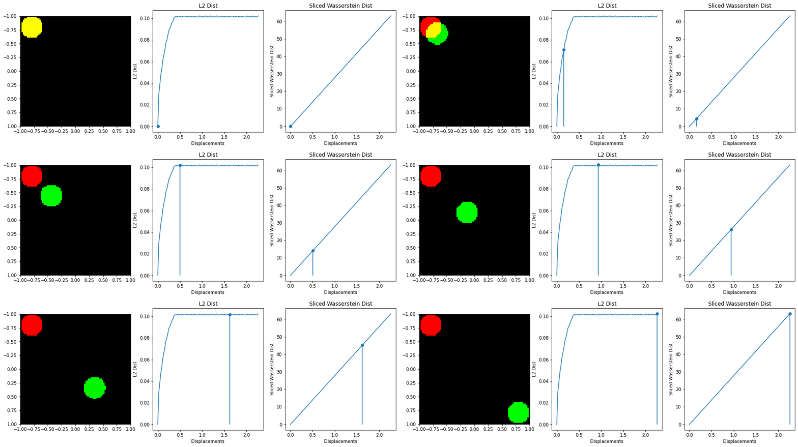
2D Histogram Sliced Wasserstein Distance via Scipy.stats
This file contains bidirectional Unicode text that may be interpreted or compiled differently than what appears below. To review, open the file in an editor that reveals hidden Unicode characters.
Learn more about bidirectional Unicode characters
| """ | |
| Original Docstring - | |
| Programmer: Chris Tralie | |
| Purpose: To use the POT library (https://github.com/rflamary/POT) | |
| to compute the Entropic regularized Wasserstein distance | |
| between points on a 2D grid | |
| Modified by Sam Mestern | |
| Shows the usage of the sliced wasserstein distance to measure the distance between two | |
| 2d histograms | |
| """ | |
| import numpy as np | |
| import matplotlib.pyplot as plt | |
| from scipy import stats | |
| def sliced_wasserstein(X, Y, num_proj): | |
| '''Takes: | |
| X: 2d (or nd) histogram | |
| Y: 2d (or nd) histogram | |
| num_proj: Number of random projections to compute the mean over | |
| --- | |
| returns: | |
| mean_emd_dist''' | |
| #% Implementation of the (non-generalized) sliced wasserstein (EMD) for 2d distributions as described here: https://arxiv.org/abs/1902.00434 %# | |
| # X and Y should be a 2d histogram | |
| # Code adapted from stackoverflow user: Dougal - https://stats.stackexchange.com/questions/404775/calculate-earth-movers-distance-for-two-grayscale-images | |
| dim = X.shape[1] | |
| ests = [] | |
| for x in range(num_proj): | |
| # sample uniformly from the unit sphere | |
| dir = np.random.rand(dim) | |
| dir /= np.linalg.norm(dir) | |
| # project the data | |
| X_proj = X @ dir | |
| Y_proj = Y @ dir | |
| # compute 1d wasserstein | |
| ests.append(stats.wasserstein_distance(np.arange(dim), np.arange(dim), X_proj, Y_proj)) | |
| return np.mean(ests) | |
| def testMovingDisc(): | |
| """ | |
| Show optimal transport on a moving disc in a 50x50 grid | |
| """ | |
| ## Step 1: Setup problem | |
| pix = np.linspace(-1, 1, 80) | |
| # Setup grid | |
| X, Y = np.meshgrid(pix, pix) | |
| # Compute pariwise distances between points on 2D grid so we know | |
| # how to score the Wasserstein distance | |
| coords = np.array([X.flatten(), Y.flatten()]).T | |
| coordsSqr = np.sum(coords**2, 1) | |
| M = coordsSqr[:, None] + coordsSqr[None, :] - 2*coords.dot(coords.T) | |
| M[M < 0] = 0 | |
| M = np.sqrt(M) | |
| ts = np.linspace(-0.8, 0.8, 100) | |
| ## Step 2: Compute L2 distances and Wasserstein | |
| Images = [] | |
| radius = 0.2 | |
| L2Dists = [0.0] | |
| WassDists = [0.0] | |
| for i, t in enumerate(ts): | |
| I = 1e-5 + np.array((X-t)**2 + (Y-t)**2 < radius**2, dtype=float) | |
| I /= np.sum(I) | |
| Images.append(I) | |
| if i > 0: | |
| L2Dists.append(np.sqrt(np.sum((I-Images[0])**2))) | |
| wass = sliced_wasserstein(Images[0], I, 1000) | |
| print(wass) | |
| WassDists.append(wass) | |
| ## Step 3: Make Animation | |
| L2Dist = np.array(L2Dists) | |
| WassDists = np.array(WassDists) | |
| I0 = Images[0] | |
| plt.figure(figsize=(15, 5)) | |
| displacements = np.sqrt(2)*(ts - ts[0]) | |
| for i, I in enumerate(Images): | |
| plt.clf() | |
| D = np.concatenate((I0[:, :, None], I[:, :, None], 0*I[:, :, None]), 2) | |
| D = D*255/np.max(I0) | |
| D = np.array(D, dtype=np.uint8) | |
| plt.subplot(131) | |
| plt.imshow(D, extent = (pix[0], pix[-1], pix[-1], pix[0])) | |
| plt.subplot(132) | |
| plt.plot(displacements, L2Dists) | |
| plt.stem([displacements[i]], [L2Dists[i]]) | |
| plt.xlabel("Displacements") | |
| plt.ylabel("L2 Dist") | |
| plt.title("L2 Dist") | |
| plt.subplot(133) | |
| plt.plot(displacements, WassDists) | |
| plt.stem([displacements[i]], [WassDists[i]]) | |
| plt.xlabel("Displacements") | |
| plt.ylabel("Sliced Wasserstein Dist") | |
| plt.title("Sliced Wasserstein Dist") | |
| plt.savefig("%i.png"%i, bbox_inches='tight') | |
| if __name__ == '__main__': | |
| testMovingDisc() |
Thanks for the snippet!
Line 38 might be problematic:
dir = np.random.rand(dim)
dir /= np.linalg.norm(dir)
since this will not give a uniform sample on a sphere. Here is an example:
import numpy as np
import matplotlib.pyplot as plt

dir = np.random.uniform(-1, 1, (20000, 2))
dir /= np.linalg.norm(dir, axis=-1, keepdims=True)

plt.scatter(dir[:, 0], dir[:, 1], alpha=0.002, edgecolors="None")
You can see that the "edges" of the uniform distribution lead to denser points in this are. While there are more elegant ways, in this case one could simply draw from a standard normal and ignore the sign which avoids the issue:
dir = np.abs(np.random.randn(dim))
dir /= np.linalg.norm(dir)
Sign up for free
to join this conversation on GitHub.
Already have an account?
Sign in to comment
Similar implementation to the author's original: https://gist.github.com/ctralie/66352ae6ab06c009f02c705385a446f3. However, uses a sliced Wasserstein metric implementation.

The sliced Wasserstein function was written by stackoverflow user dougal - https://stats.stackexchange.com/questions/404775/calculate-earth-movers-distance-for-two-grayscale-images
Reference: https://link.springer.com/article/10.1007/s10851-014-0506-3