Draw a neural network diagram with matplotlib!

draw_neural_net.py

import matplotlib.pyplot as plt

def draw_neural_net(ax, left, right, bottom, top, layer_sizes):
    '''
    Draw a neural network cartoon using matplotilb.
    
    :usage:
        >>> fig = plt.figure(figsize=(12, 12))
        >>> draw_neural_net(fig.gca(), .1, .9, .1, .9, [4, 7, 2])
    
    :parameters:
        - ax : matplotlib.axes.AxesSubplot
            The axes on which to plot the cartoon (get e.g. by plt.gca())
        - left : float
            The center of the leftmost node(s) will be placed here
        - right : float
            The center of the rightmost node(s) will be placed here
        - bottom : float
            The center of the bottommost node(s) will be placed here
        - top : float
            The center of the topmost node(s) will be placed here
        - layer_sizes : list of int
            List of layer sizes, including input and output dimensionality
    '''
    n_layers = len(layer_sizes)
    v_spacing = (top - bottom)/float(max(layer_sizes))
    h_spacing = (right - left)/float(len(layer_sizes) - 1)
    # Nodes
    for n, layer_size in enumerate(layer_sizes):
        layer_top = v_spacing*(layer_size - 1)/2. + (top + bottom)/2.
        for m in xrange(layer_size):
            circle = plt.Circle((n*h_spacing + left, layer_top - m*v_spacing), v_spacing/4.,
                                color='w', ec='k', zorder=4)
            ax.add_artist(circle)
    # Edges
    for n, (layer_size_a, layer_size_b) in enumerate(zip(layer_sizes[:-1], layer_sizes[1:])):
        layer_top_a = v_spacing*(layer_size_a - 1)/2. + (top + bottom)/2.
        layer_top_b = v_spacing*(layer_size_b - 1)/2. + (top + bottom)/2.
        for m in xrange(layer_size_a):
            for o in xrange(layer_size_b):
                line = plt.Line2D([n*h_spacing + left, (n + 1)*h_spacing + left],
                                  [layer_top_a - m*v_spacing, layer_top_b - o*v_spacing], c='k')
                ax.add_artist(line)

Thanks for the example @craffel!
In case anybody else wants a quick preview, here's the image the code produces.

I removed the axis with:

fig = plt.figure(figsize=(12, 12))
ax = fig.gca()
ax.axis('off')
draw_neural_net(ax, .1, .9, .1, .9, [4, 7, 2])
fig.savefig('nn.png')

@bamos and thanks to you for the example :)!

How can I write something into a neuron?

@craffel Very useful, thank you!
@kanban1992 I wanted to do the same, so I forked this and added node annotation functionality.

Great job. Thanks.

Thanks a lot.

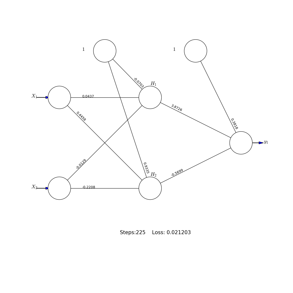
Besides, based on your smart codes, I attempt to add texts of Inputs (X_1,X_2,...,H_1, H_2,..., y_1,y_2,...) and bias nodes(labeled as '1') and
the edges (lines) between bias and nodes. Furthermore, the weights (coefs_ and intercepts_ executed after MLPClassifier) are
marked along the edges (using plt.text with orientation). Finally, add the information (n_iter_ and loss_) below the topology.

The function for plotting the network are as follows:

#---------------------------------------------------------------------

filename: [draw_neural_net_.py]

#---------------------------------------------------------------------
def draw_neural_net(ax, left, right, bottom, top, layer_sizes,
coefs_,
intercepts_,
n_iter_,
loss_,
np, plt):
'''
Draw a neural network cartoon using matplotilb.

:usage:
    >>> fig = plt.figure(figsize=(12, 12))
    >>> draw_neural_net(fig.gca(), .1, .9, .1, .9, [4, 7, 2])

:parameters:
    - ax : matplotlib.axes.AxesSubplot
        The axes on which to plot the cartoon (get e.g. by plt.gca())
    - left : float
        The center of the leftmost node(s) will be placed here
    - right : float
        The center of the rightmost node(s) will be placed here
    - bottom : float
        The center of the bottommost node(s) will be placed here
    - top : float
        The center of the topmost node(s) will be placed here
    - layer_sizes : list of int
        List of layer sizes, including input and output dimensionality
    - coefs_ :(list) length (n_layers - 1) The ith element in the list represents the weight matrix corresponding to layer i.
    - intercepts_ : (list) length (n_layers - 1)The ith element in the list represents the bias vector corresponding to layer i + 1.
    - n_iter_ : (int) The number of iterations the solver has ran.
    - loss_ : (float) The current loss computed with the loss function.
'''
n_layers = len(layer_sizes)
v_spacing = (top - bottom)/float(max(layer_sizes))
h_spacing = (right - left)/float(len(layer_sizes) - 1)
# Input-Arrows
layer_top_0 = v_spacing*(layer_sizes[0] - 1)/2. + (top + bottom)/2.
for m in xrange(layer_sizes[0]):
    plt.arrow(left-0.18, layer_top_0 - m*v_spacing, 0.12, 0,  lw =1, head_width=0.01, head_length=0.02)
# Nodes
for n, layer_size in enumerate(layer_sizes):
    layer_top = v_spacing*(layer_size - 1)/2. + (top + bottom)/2.
    for m in xrange(layer_size):
        circle = plt.Circle((n*h_spacing + left, layer_top - m*v_spacing), v_spacing/8.,\
                            color='w', ec='k', zorder=4)

plt.plot(nh_spacing + left, layer_top - mv_spacing, 'o', mfc='w', mec='k', ls= '-', markersize = 40)

# Add texts
        if n == 0:
            plt.text(left-0.125, layer_top - m*v_spacing, r'$X_{'+str(m+1)+'}$', fontsize=15)
        elif (n_layers == 3) & (n == 1):
            plt.text(n*h_spacing + left+0.00, layer_top - m*v_spacing+ (v_spacing/8.+0.01*v_spacing), r'$H_{'+str(m+1)+'}$', fontsize=15)
        elif n == n_layers -1:
            plt.text(n*h_spacing + left+0.10, layer_top - m*v_spacing, r'$y_{'+str(m+1)+'}$', fontsize=15)
        ax.add_artist(circle)# 
# Bias-Nodes
for n, layer_size in enumerate(layer_sizes):
    if n < n_layers -1:
        x_bias = (n+0.5)*h_spacing + left
        y_bias = top + 0.005
        circle = plt.Circle((x_bias, y_bias), v_spacing/8.,\
                            color='w', ec='k', zorder=4)
# Add texts
        plt.text(x_bias-(v_spacing/8.+0.10*v_spacing+0.01), y_bias, r'$1$', fontsize=15)
        ax.add_artist(circle)   
# Edges between nodes
for n, (layer_size_a, layer_size_b) in enumerate(zip(layer_sizes[:-1], layer_sizes[1:])):
    layer_top_a = v_spacing*(layer_size_a - 1)/2. + (top + bottom)/2.
    layer_top_b = v_spacing*(layer_size_b - 1)/2. + (top + bottom)/2.
    for m in xrange(layer_size_a):
        print(m)
        for o in xrange(layer_size_b):
            line = plt.Line2D([n*h_spacing + left, (n + 1)*h_spacing + left],
                              [layer_top_a - m*v_spacing, layer_top_b - o*v_spacing], c='k')
            ax.add_artist(line)
            xm = (n*h_spacing + left)
            xo = ((n + 1)*h_spacing + left)
            ym = (layer_top_a - m*v_spacing)
            yo = (layer_top_b - o*v_spacing)
            rot_mo_rad = np.arctan((yo-ym)/(xo-xm))
            rot_mo_deg = rot_mo_rad*180./np.pi
            xm1 = xm + (v_spacing/8.+0.05)*np.cos(rot_mo_rad)
            if n == 0:
                if yo > ym:
                    ym1 = ym + (v_spacing/8.+0.12)*np.sin(rot_mo_rad)
                else:
                    ym1 = ym + (v_spacing/8.+0.05)*np.sin(rot_mo_rad)
            else:
                if yo > ym:
                    ym1 = ym + (v_spacing/8.+0.12)*np.sin(rot_mo_rad)
                else:
                    ym1 = ym + (v_spacing/8.+0.04)*np.sin(rot_mo_rad)
            plt.text( xm1, ym1,\
                     str(round(coefs_[n][m, o],4)),\
                     rotation = rot_mo_deg, \
                     fontsize = 10)
# Edges between bias and nodes
for n, (layer_size_a, layer_size_b) in enumerate(zip(layer_sizes[:-1], layer_sizes[1:])):
    if n < n_layers-1:
        layer_top_a = v_spacing*(layer_size_a - 1)/2. + (top + bottom)/2.
        layer_top_b = v_spacing*(layer_size_b - 1)/2. + (top + bottom)/2.

for m in xrange(layer_size_a):

        x_bias = (n+0.5)*h_spacing + left
        y_bias = top + 0.005 
        for o in xrange(layer_size_b):
            print(o)
            line = plt.Line2D([x_bias, (n + 1)*h_spacing + left],
                          [y_bias, layer_top_b - o*v_spacing], c='k')
            ax.add_artist(line)
            xo = ((n + 1)*h_spacing + left)
            yo = (layer_top_b - o*v_spacing)
            rot_bo_rad = np.arctan((yo-y_bias)/(xo-x_bias))
            rot_bo_deg = rot_bo_rad*180./np.pi
            xo2 = xo - (v_spacing/8.+0.01)*np.cos(rot_bo_rad)
            yo2 = yo - (v_spacing/8.+0.01)*np.sin(rot_bo_rad)
            xo1 = xo2 -0.05 *np.cos(rot_bo_rad)
            yo1 = yo2 -0.05 *np.sin(rot_bo_rad)
            plt.text( xo1, yo1,\
                 str(round(intercepts_[n][o],4)),\
                 rotation = rot_bo_deg, \
                 fontsize = 10)    
# Output-Arrows
layer_top_0 = v_spacing*(layer_sizes[-1] - 1)/2. + (top + bottom)/2.
for m in xrange(layer_sizes[-1]):
    plt.arrow(right+0.015, layer_top_0 - m*v_spacing, 0.16*h_spacing, 0,  lw =1, head_width=0.01, head_length=0.02)
# Record the n_iter_ and loss
plt.text(left + (right-left)/3., bottom - 0.005*v_spacing, \
         'Steps:'+str(n_iter_)+'    Loss: ' + str(round(loss_, 6)), fontsize = 15)

#----------------------------------------------------------------------------------------------------------------------------------

The testing main program is:
#========================================

filename: [test_XOR_Classification.py]

#--------------------------------------------------------------------
import numpy as np
import matplotlib.pyplot as plt
from sklearn.neural_network import MLPClassifier as MLP
from draw_neural_net_ import draw_neural_net

#--------[1] Input data
dataset = np.mat('-1 -1 -1;
-1 1 1;
1 -1 1;
1 1 -1')
#----------------------------------------------------

(You should define the X_train and y_train

#----------------------------------------------------

testing different topology

#----------------------------------------
#-----2-2-1
my_hidden_layer_sizes= (2,)
#------2-2-8-1
#my_hidden_layer_sizes= (2, 8,)
#------2-16-16-1
#my_hidden_layer_sizes= (16, 16,)

XOR_MLP = MLP(
activation='tanh',
alpha=0.,
batch_size='auto',
beta_1=0.9,
beta_2=0.999,
early_stopping=False,
epsilon=1e-08,
hidden_layer_sizes= my_hidden_layer_sizes,
learning_rate='constant',
learning_rate_init = 0.1,
max_iter=5000,
momentum=0.5,
nesterovs_momentum=True,
power_t=0.5,
random_state=0,
shuffle=True,
solver='sgd',
tol=0.0001,
validation_fraction=0.1,
verbose=False,
warm_start=False)
#----------[2-2] Training
XOR_MLP.fit(X_train,y_train)
#-----------------------------------------------------------

plot the neural network

#-----------------------------------------------------------

fig66 = plt.figure(figsize=(12, 12))
ax = fig66.gca()
ax.axis('off')

draw_neural_net(ax, .1, .9, .1, .9, [2, 2, 1],
XOR_MLP.coefs_,
XOR_MLP.intercepts_,
XOR_MLP.n_iter_,
XOR_MLP.loss_,
np, plt)
plt.savefig('fig66_nn.png')
#=========================================

Topology: 2-2-1

Topology: 2-2-8-1

Topology: 2-16-16-1

The result hadn't been tuned to the best. Only for demonstrating the plotting network topology using sklearn and matplotlib in Python.
You can tune the parameters of MLPClassifier and test another examples with more inputs (Xs) and outputs (Ys) such as IRIS (X1--X4, Y1--Y3).

Thanks for the script!
Btw, does this work for both Python 2 and 3? I'd like to suggest specifying it in some kind of comment or a shebang.

Suppose that it can work in Python 2 and Python 3. Here, I employ Python 2.7 to test it. You can try to execute it. You also can modify the X_labels to be the real names (such as from 'X_1', 'X_2' to 'Sepal.Length', 'Sepal.Width'and from y_1, y_2, y_3 to 'Setosa', 'Versicolor' and 'Virginica' by adding some plot.text() commands.

@ljhuang2017 do you have that file available somewhere else? looks like the formatting got kind of borked.

@ljhuang2017 this looks very nice. Could you just make another gist out of it? Just edit your comment, copy your code and paste it in a new gist. This way people can use your code without the need of reformating it.

I don't think people are notified when you @ them on Gists, and @ljhuang2017 doesn't have any contact information. Did anyone get their code working? Can you post it as your own Gist if so?

Many thanks for the script!

I was able to successfully run @ljhuang2017 code and posted on a new gist
The final result looks like this:

Thank you for the code, saved me a lot of time drawing it myself.

How can i have labels for coefficients and intercepts. I need for demonstration.

Labels(a1,b1,c1,d1 ) etc.. like this

@craffel Thanks for the wonderful code. However, the layers get added from top to bottom, not from left to right. This makes me find difficulties in putting separate colors for the nodes in the input, hidden layer, and output! Could that be done? Also, some annotations for the layers?

Halu, I wanted to use these codes, but since I use python3 I needed to change some stuff to make it work.

Thus, I did some minor changes to @dvgodoy gist code, so now it supports python3 and np.array()

link