-
-
Save heejongahn/00d68a40415613893ad0 to your computer and use it in GitHub Desktop.
| 우하하 |
Processor I : Datapath and Control
Clocking methodology
결국 프로그램은 다음과 같은 과정의 반복이다:
state elements의 현재 컨텐츠를 읽어옴 -> combinational logic -> 결과값을 하나
이상의 state element에 씀
이 때 write는 clock signal이 들어오는 clock edge에서만 이루어진다. 그렇지 않을
경우 읽어오는 값이 정말 원하는 그 값이라는 것을 보증할 수가 없음!
Datapath
CPU에서 데이터 / 주소를 처리하는 레지스터, ALU, mux, memory 등등이 모두
datapath. 간단한 데이터패스에서부터 시작해 점점 증가시켜보자.
일단 기본적으로 다음과 같은 과정을 생각해보자:
Fetching instructions
Instruction Memory 로부터 인스트럭션을 읽어 옴, PC update. 이 때 PC는 매 클락 사이클마다 업데이트 되어야 하므로 따로 write signal을 필요로 하지 않는다.
마찬가지로 IM에서 읽어오는 일도 explicit read signal을 필요로 하지 않음.
Decoding Instructions
위에서 fetch된 인스트럭션의 opcode + function field를 control unit에게 전달. 이를 이용해 fetch된 인스트럭션이 어떤 인스트럭션인지를 특정할 수 있다. 또한, (최대 두 개의) 값을 레지스터 파일로부터 읽어온다.
Executing R Format Operations
rs, rt 레지스터의 값을 이용해 명령어를 실행한 뒤 결과값을 rd에 wirte back. 이 때 레지스터 파일의 write back은 이루어지지 않는 경우도 있으니 (ex: sw) explicit write signal을 필요로 한다.
ALU는 레지스터 파일로부터 2개의 값을 받아올 수 있어야 하며, ALU control 신호를 받고 overflow / zero flag를 내보낸다. 그리고 레지스터 파일로 1개의 값을 쓸 수 있어야 함.
Executing Load and Store Operations
베이스 레지스터값 + 16비트 signed-extended offset 의 결과값 주소를 계산할 수 있어야 함. 그 뒤 그 주소에 쓰거나(store) 그 주소로부터 읽어옴(load).
레지스터 파일을 거치지 않고 인스트럭션에서 바로 ALU로 가는 immediate path가 필요함 (sign extend). 또한, 데이터 메모리가 데이터패스에 추가된다.
Executing Branch Operations
ALU의 결과 zero flag를 받는 branch controller 필요. 인스트럭션의 immediate field를 shift left 2 한 값과 PC를 더해서 branch target address로 사용.
Executing Jump Operations
target PC = (upper 4 bits of current PC) + (26 bits immediate field) + 00
Creating a Single Datapath
위에서 나온 datapath segment들을 조합해서 데이터패스를 만들어보자! 현재로서는 Single cycle design을 사용 : 모든 인스트럭션에 대한 fetch, decode, exectution 까지가 1 clock cycle 내에 마쳐짐.
- 하나의 리소스가 하나의 인스트럭션 당 한 번 이상 사용될 수 없으므로 여러 중복된 리소스들이 생김. 예를 들어, Instruction Memory와 Data Memory가 분리되고, adder가 여러개 존재.
- 두 개 이상의 인풋이 들어올 수 있는 곳에는 multiplexor가 필요함.
- 레지스터 파일, 데이터 메모리에 대한 쓰기를 제어하기 위해 write signal이 필요함.
가장 긴 경로에 의해 cycle time이 결정된다.
Controller
ALU, 레지스터 파일, 메모리 읽기/쓰기 등의 명령을 시행할 지 말지를 결정함. 데이터의 흐름을 제어.
- 상위 6비트는 무조건 opcode
- 읽을 레지스터는 무조건 rs(source), rt field에 들어있음. lw/sw의 경우 rs가 base
register. - 쓸 레지스터는 lw의 경우 rt에, R-type 인스트럭션의 경우 rd(destination)에 들어있음.
ALU Control
- Add : load / store (base register + offset)
- Subtract : branch (target address - (PC + 4))
- Depends : R type's function field
opcode로부터 나오는 2bit ALUOp + function field로 ALU Control 정해짐.
- ALUOp 가 00 / 11 (lw, sw, beq) : function field와 무관하게 ALU control 각각
0010(add) 혹은 0110(subtract)로 정해짐. - ALUOp가 10 (R-type) : function field와 조합해서 정해짐.
Control Signal 생성법
Microcoded control
프로세서 내의 조그만 부분에 컨트롤 시그널이 정의되어 있음. 느림.
Hardwired control
combinational logic 내에서 컨트롤 시그널 생성. RISC에서 사용.
Processor II : Pipeline
Instruction time
Single cycle design 의 특징:
- 가장 오래 걸리는 인스트럭션보다 약간 더 긴 시간이 clock cycle time이 된다.
보통 load instruction. - 한 클락 사이클 동안 하나의 리소스를 동시에 쓸 수 없기 때문에 adder를 비롯한 functional unit 들이 중복되어 필요하다.
- 간단하고, 이해하기 쉽다.
Performance Issue
- 가장 긴 인스트럭션 (critical path : load instruction) 이 clock period를
결정한다. - 다른 인스트럭션들에 대해 period를 다르게 줄 수 없다.
- 디자인 원칙 (Make the common case fast) 를 위배한다.
Pipeline to the rescue!
인스트럭션을 받아와서 해석하고 실행하고 결과를 저장하는 과정들을 작은 가정들로
쪼갠다. 그 이후에 하나의 인스트럭션이 끝나기 전에 그 다음 인스트럭션을 실행.
이상적인 조건 - 각 단계의 실행에 걸리는 시간이 동일 - 이 만족될 경우,
(speedup of pipelining) = (number of pipe stages)
The Five Stages of Load Instruction
- IFetch : Instruction Fetch + PC Update
- Decoding : Registers Fecth + Instruction Decoding
- Execution : Execute R-type + calcuate memory address
- Memory : Read/write the data from/to the Data Memory
- Write Back : Write the result data into the register file
Benefits of Pipelining
- 파이프라인 이전 : CPI 1 (single cycle design), long cycle clock time
- 파이프라인 이후 : CPI 1 (ideally), 훨씬 짧은 cycle clock time
파이프라이닝은
- 각 작업의 latency를 줄여주지 않는다. 대신 전체 workload의 throughput을 improve
- 서로 다른 리소스를 사용하는 여러 작업들을 simultaneously 실행
- 가장 느린 단계에 의해서 pipeline rate가 결정됨 -> 단계별 소모시간 차이가
적을수록 효율적
Pipelining and ISA Design
MIPS ISA과 파이프라이닝
- 모든 인스트럭션이 32비트 -> 한 사이클 내에 fetch & decode 하기에 좋다
- 비교적 간단한 일만을 하는, 적은 종류의 인스트럭션 -> 한 사이클 내에 decode &
read register 하기에 좋다 - Load/Store의 타겟 주소는 3단계(Exec)의 ALU를 거치고 난 뒤 결정되고 메모리
접근은 4단계에서 - aligned memory -> 메모리 접근도 한 사이클 내에 가능
MIPS Pipeline Datapath - Addition and Modification
Addition : Latch
각 단계를 분리하기 위해 IF/ID, ID/EX, EX/MEM, MEM/WB 각각 상태를 저장하는 state
register(latch)가 필요하다.
Modification
모든 Control signal은 Decode 단계에서 결정되고, 위에서 추가된 latch에 저장된다.
Basics of Digital Logic
high voltage -> logical 1, low voltage -> logical 0
Combinational Logic
The output depends only on current inputs - truth table
Logic element 로는 AND(out = A•B), OR(out = A+B), NOT(out = ~A)
AND(둥글이), OR(뾰족이), NOT(삼각이)
Laws of Boolean Algebra
- Identity law : A+0 = A•1 = A
- Zero and One laws : A+1 = 1, A•0 = 0
- Inverse laws : A+(~A) = 1, A•(~A) = 0
- Commutative laws = A+B = B+A, A•B = B•A
- Associative laws = A+(B+C) = (A+B)+C, A•(B•C) = (A•B)•C
- Distributive laws = A•(B+C) = A•B+A•C, A+(B•C) = (A+B)•(A+C)
- DeMorgan's laws = ~(A+B) = (~A)•(~B), ~(A•B) = (~A)+(~B)
증명은 truth table로 간단히 할 수 있다.
Truth table -> Logic Equation
Sum of products : truth table에서 out이 1인 녀석들을 싸그리 OR 연산
NAND 혹은 NOR만 있으면 어떤 combinational logic도 다 만들수 있다.
Decoder
input: n-bit, output: pow(2, n)
인풋을 보고 총 2의 n승개의 output 중 하나만 activate
Multiplexer
2개 (혹은 여러개) 의 인풋이 들어올 때 control signal을 보고 하나만 선택
Full adder
A, B, Carry In 3비트 인풋 -> Sum, Carry Out 2비트 아웃풋
회로
Four Bit Adder
4비트 가산기를 만들기 위해서는 4개의 전가산기가 필요하답니다.
Sequential Logic
combinational logic 과는 다르게, sequential circuit의 아웃풋은 current input은
물론, past input 들에도 의존한다. 따라서 상태를 저장할 수 있는 element - memory
element 가 필요하다.
Clock
State 는 clock edge 에서만 업데이트된다 (edge-triggered clocking)
Latch
간단한 memory element.
D Latch :data value D + clock signal C -> output Q. Clock edge에서만 값이 변한다.
Register
n-bit 레지스터 : 병렬로 연결된 n개의 flip-flop.
레지스터 파일 : 레지스터 넘버로 접근 가능한 레지스터의 집합
Computer Elements
Transistor
스위치로서 사용된다.
- 0(False) = V < V_lo
- 1(True) = V > V_hi
- in between = Forbidden
MOS Transistor, CMOS, ...
Skip
이상과 현실의 차이
CS 하는 사람들은 인풋의 변화가 아웃풋에 즉각 반영되길 원하지만 실제로 회로는
그렇게 돌아가지 않는단다. 그래서 클락이란게 필요해용!
- Setup TIme : clock edge 전에 인풋이 stable 해야 함
- Hold Time : clock edge 이후에 인풋이 stable 해야 함
Critical path
두개의 저장장치 사이의 가장 느린 경로. cycle time 은 critical path 를 가는데에
걸리는 시간에 직접적으로 의존한다.
Clock-to-Q + Longest Path through the Combinational Logic + Setup < Cycle Time
How to reduce cycle time?
- gate level의 수를 줄인다
- multiple stages to drive large load
Memory
SRAM vs DRAM
SRAM
- fast but expensive
- 1 control liine, 2 data lines
DRAM
- better density
- need periodic refresh
- reads are destructive
Pipeline Hazard
Pipeline Hazard
- Structural Hazard
- Data Hazard
- Control Hazard
Structural Hazard
같은 리소스를 동시에 두 개의 인스트럭션이 사용하려 할 때 발생
예: store과 instruction fetch가 같은 메모리에 대해 일어난다.
Data Hazard
어떤 데이터가 준비되기 전에 (e.g. 이전에 실행되어야 할 쓰기가 완료되기 전에)
사용하려 할 때 발생.
add $1, $2, $3
add $5, $1, $2
이 경우 $1에 올바른 값이 쓰여지기 전에 다음 인스트럭션에서 읽어버림
Control Hazard
beq, bne, j, jal 같은 conditional/unconditional jump가 있을 시 바로 뒤에
fetch 해 왔던 인스트럭션이 쓸모 없어질 수 있음.
The easiest solution
-> bubble(stall)
Concrete Examples
Single memory
lw와 IF가 동시에 일어나면서 같은 메모리에 접근
-> 인스트럭션 / 데이터 메모리 분리로 해결 가능
Register File Access
동시에 같은 레지스터 파일에 읽고 쓰는 두 인스트럭션이 있을 수 있다
레지스터 파일에 대한 쓰기는 first half에, 읽기는 second half에만 하면 해결
dependency backward는 data harard로 이어진다
add $1,
sub $4, $1,
and $6, $1,
Read before write data hazard
lw $1, 4($2)
sub $4, $1,
and $6, $1,
Load-use data hazard
Branch Instruction
beq ...
adsf
control hazard
Let's 'FIX' data hazards
- Stall : impacts CPI
- Forwarding : ALU의 연산 결과를 Register file로, EX/MEM 혹은 MEM/WB 결과를
ALU로, ...
EX Forward Unit
if (EX/MEM.RegWrite
and (EX/MEM.RegisterRd != 0)
and (EX/MEM.RegisterRd = ID/EX.RegisterRs))
  ForwardA = 10

if (EX/MEM.RegWrite
and (EX/MEM.RegisterRd != 0)
and (EX/MEM.RegisterRd = ID/EX.RegisterRt))
  ForwardB = 10
MEM Forward Unit
if (MEM/WB.RegWrite
and (MEM/WB.RegisterRd != 0)
**and (EX/MEM.RegisterRd != ID/EX.RegisterRs)**
and (MEM/WB.RegisterRd = ID/EX.RegisterRs))
  ForwardA = 01

if (MEM/WB.RegWrite
and (MEM/WB.RegisterRd != 0)
**and (EX/MEM.RegisterRd != ID/EX.RegisterRt)**
and (MEM/WB.RegisterRd = ID/EX.RegisterRt))
  ForwardB = 01
Code Scheduling
똑같은 일을 하는 코드 상에서 어셈블리 순서를 바꿈으로서 stall을 피해갈 수 있다.
MEM to MEM Copy
load 바로 뒤에 store이 나오는경우, MEM/WB 레지스터를 data memory로
포워딩함으로서 stall을 피할 수 있다.
Load-use
lw 한 레지스터를 사용하기 위해서는 적어도 하나의 stall이 필요하다.
if (ID/EX.MemRead
and ((ID/EX.RegisterRt = IF/ID.RegisterRs)
or (ID/EX.RegisterRt = IF/ID.RegisterRt))
stall the pipeline
Hazard/Stall HW
Stall을 실제로 어떻게 구현하는가? -> PC register + IF/ID pipeline register를
보존 (Hazard detection unit이 PC.write 및 IF/ID.write 제어)
EX stage의 _lw_와 ID stage의 load-use instruction 사이에 "bubble(noop)"을
집어넣음.
Pipeline Control Hazard
Control Hazard
인스트럭션 주소가 sequential하게 (PC = PC + 4) 흐르지 않을 때 발생.
- Uncondtional branches (j, jal, jr)
- Conditional branches (beq, bne)
- Exceptions
가능한 해결책들
- Stall
- 분기의 방향을 최대한 빠르게 옮긴다
- Delay decision (컴파일러 도움 필요)
- 분기 예측
데이터 해저드의 forwarding 처럼 무조건 좋은 녀석은 없다.
Unconditional branch
ID(Decoding) stage 가 지나야 jump 임을 알 수 있음
-> 하나의 flush가 필요함. IF.Flush = 0 (j 바로 다음 인스트럭션을 noop으로 만듬)
두 종류의 Stall
- bubble : 버리는 인스트럭션 없음. 파이프라인에서 두 인스트럭션 사이에 noop을 끼워넣는다.
- flush : 파이프라인에서 이미 들어온 인스트럭션을 noop으로 바꿔버림.
Conditional branch
Flushing
beq
lw
inst 3
inst 4
가 있다고 해보자. beq의 타겟 주소는 MEM stage 이후에 알 수 있으므로 3개의
인스트럭션을 flush 해야 함 -> CPI에서 심각한 손해를 봄.
Early decision
만약 ID 혹은 EX stage 에서 branch target을 알 수 있다면 그만큼 적은 stall을
필요로 한다.
이 때 추가적인 HW compent (mux, AND gate, adder, ...) 들을 필요로 함.
ID Branch Forwarding Issues
앞의 단계에서 branch target 계산을 위해서는 앞의 인스트럭션에서의 결과값을
넘겨줘야 할 때가 있다.
이 때, branch instruction이 execute 되는 시점에서 올바른 값을 갖고 있음이 보장되어야
한다. 만약 직전 인스트럭션의 rd가 branch target을 결정하는 레지스터 중 하나라면
stall이 필요하다.
Static Branch Prediction
정적으로 분기를 예측해보자.
Predict not taken
항상 분기가 택해지지 않는다고 가정하고 sequential 한 인스트럭션들을 fetch.
보동 top of the loop branching structure 에서 잘 동작한다. (끝까지 내려간 뒤에
맨 위로 j하고 beq 일시 break하는 구조)
bottom of the loop branching structure 에서는 잘 동작하지 않는다.
Predict taken
항상 1개의 stall cycle이 존재한다.
Dynamic Branch Prediction
IF stage에 BHT(branch history table)이 존재, 어떤 주소의 branch가 지난 실행에서
택해졌는지 아닌지에 대한 정보를 갖고 있다. 이 prediction은 틀려도 correctness에는
영향을 주지 않고 performance 만 깎아먹음.

Branch Target Buffer
BHT로는 branch take 여부만 알 수 있지, target을 알 수 없다.
따라서 IF stage cache에 branch target buffer(BTB)를 둬서 branch target address를
저장. Two read port instruction memory 가 필요하다.
2-bit Predictor
2번 틀려야만 예측 방향을 바꾸게 한다.

Exceptions
다양한 소스에서부터 오는 예외들을 어떻게 처리해줘야 할까? 크게 다음과 같이 두
종류로 나눌 수 있다.
- Interrupts (asynchronous) : caused by external events
I/O service requets, HW malfunction, ... - Traps (synchronous) : caused by internal events
Arithmetic overflow, Undefined instruction, ...
single clock cylce 내에서도 여러 예외가 동시에 일어날 수 있다. 이 때 HW가 알아서
소팅해준 뒤에 가장 먼저 fetch 된 인스트럭션의 예외부터 처리한다.
HW
- Cause Register : 예외의 원인 기록
- EPC Register : 예외가 일어난 PC 기록
Memory Hierachy: Cache Basics
Memory Hierarchy
Memory Technology
- Static RAM : 매우 빠르지만 컴포넌트가 많아 density 떨어짐. cost per byte 매우
높다. 전력 소모 큼. - Dynamic RAM : dense 하지만 상대적으로 느리다.
- Magnetic disk : 매우 느리고 엄청나게 싸다
우리는 SRAM의 속도와 자기 디스크의 가성비를 가진 저장 장치를 원한다. 도둑놈 심보
Memory Hierarchy Technology
- SRAM for cache : speed, tech compatibility
- DRAM for main memor : 보다 느리지만 괜찮은 속도, 높은 밀집도. 주기적으로
capacitor를 refresh 시켜줘야 한다.
Processor-Memory Performance Gap
Microprocessor의 성능은 무어의 법칙에 따라 18개월마다 2배 정도의 성장세를 보이는데,
메인 메모리 성능은 그 성장세를 전혀 못 따라가고 있다.
우리의 pipeline design은 메모리 접근에 1 cycle access로 충분하다고 가정하지만,
실제로 main memory access time은 200 cycle 정도.
Hierarchy + parallelism = The illusion of large, fast and cheap memory!
Locality
Locality
Locality
정말 중요하니까 세 번 썼다. 이걸 이용해서 위에서 말한 환상을 만들어냄.
- register <-> memory : 컴파일러가 관리
- cache <-> main memory : 캐시 컨트롤러 HW가 관리
- main memory <-> disk : OS가 관리 (가상 메모리) w/ TLB
Locality
- Temporal (time)
- Spatial (space)
뭔지는 다 알거라 믿는다. 얼마나 locality를 잘 살린 프로그램을 짜느냐는 1차적으로프로그래머의 몫.
Terminology
- Block
- Hit Rate, Hit Time (블락까지 가는 시간 + Hit인지 판별하는 시간)
- Miss Rate, Miss Penalty (Miss일 때 갈아끼는 시간)
Example
70% hit rate, cache hit 1 cycle, main memory access 25 cycle.
Average memory access time = Hit Latency + Miss rate * Miss Latency = 1 + (0.3) * 25 = 8.5
Cache Basics
- 찾는 데이터가 캐시에 있는가?
- 있다면, 캐시 속 어디에 있는가?
Direct Mapping : memory block은 단 하나의 cache block에만 매핑 된다. 주소의 upper portion을 캐시 테이블의 인덱스로 사용.
Basic Structure
concrete (multiword) example: 4B word, 4KB cache, 16B per line
32-bit address -> 2-bit byte offset + 2-bit block offset + 8-bit index + 20-bit
tag
- Direct Mapped Cache : Temporal locality
- Multiword Block Direct Mapped Cache : Temporal + Spatial locality
Tradeoffs
Block size가 커질 때
- Spatial locality 증가
- 블락 개수가 줄어듬 -> more competition
- miss penalty가 커짐 (더 큰 블락을 가져와야 함)
블락 사이즈가 커짐에 따라 miss rate는 줄어들다가 어느 수준을 넘어서면 커짐. 너무큰 블락 사이즈로는 캐시에 블락이 몇 개 밖에 못 올라와있음.
Instruction Set Architectue I
Instruction Set Architecture
Contract between programmer and the HW
- 프로그래머 : 프로그램이 어떻게 실행될지에 대한 모델
- HW 디자이너 : 프로그램을 올바르게 실행하는 방법에 대한 formal definition
우리는 MIPS를 사용할거야.
Two Key Principles
- 인스트럭션이랑 데이터 구분 불가
- 데이터처럼 프로그램도 메모리에 올라감
state -> formatted instruction -> another state
Design principle 1: Siplicity favors regularity
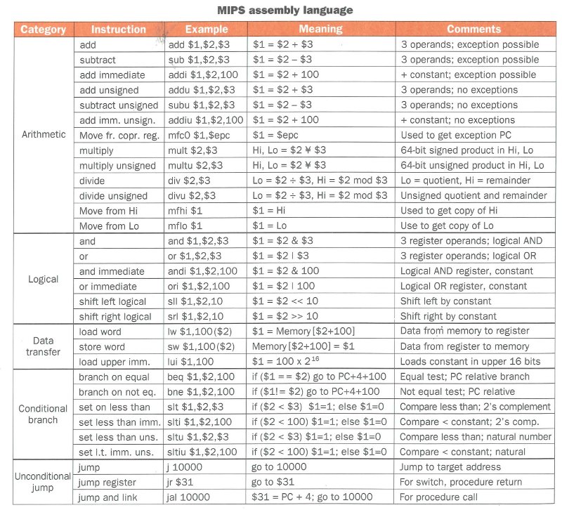
MIPS-32 ISA
Arithmetic Instructions
instruction rd, rs, rt -> rd = rs (instruction) rt
formatted as opcode | rs | rt | rd | shamt | function
f = (g + h) - (i + j);
MIPS (pseudo)코드로 쓰면
add t0, g, h
add t1, i, h
sub f, t0, t1
MIPS는 Big Endian : MSB가 가장 낮은 주소에!
Design principle 2: Smaller is faster
MIPS Register File
32개의 32-bit register가 들어있음. 2개의 읽기 포트, 1개의 쓰기 포트.
레지스터의 특징
- 메인 메모리보다 빠르다. 이 때 레지스터 개수 혹은 포트수가 늘어나면 느려짐
- 컴파일러가 사용하기 쉽다
- 변수를 여기 저장하면 코드 밀집도가 증가함 (메모리 주소보다 적은 공간 차지)
Types of operand
- Register operand: $0(zero), $5, ... -> 매우 빠르다
- Memory operand: offset(base register) = (base register 값 + offset) 위치에 있는 데이터
- immediate openand: 상수값. 작은 상수들은 자주 쓰이니까 이걸 이용해서 계산하렴.
Design principle 3: Make the common case fast
zero register($0) 상수 0으로 고정. 레지스터간 값 이동등에 사용하렴.
signed extension, unsigned integer, 2's complement -> 생략
MIPS Instruction formats

Design principle 4: Good design demands good compromises
Instructions
If statement
if (i==j) f = g+h;
else f = g-h;
f가 $4에, g가 $5에, h가 $6에 있다 치면
      bne $5, $6, Else
      add $4, $5, $6
      j Exit
Else: sub $4, $5, $6
Exit: ...
Loop statement
while (save[i] == k) i += 1;
i가 $3에, k가 $5에, save의 주소가 $6에 있다 치면
Loop: sll $1, $3, 2
      add $1, $1, $6
      lw  $2, 0($1)
      bne $2, $5, Exit
      addi $3, $3, 1
      j Loop
Exit: ...
Basic blocks
브랜치나 브랜치 타겟 없이 무조건 같이 실행되는 블락. 컴파일러는 최적화를 위해
basic block을 구분한다.
Why not blt, bge, ...?
-> 대소 비교를 위한 HW가 같은지 아닌지 비교하는 애보다 훨씬 느리다. Faster
common cases!
Instruction Set Architecture II
Procedure call
메모리 중 Stack에 쌓인다. 각 프로시져 콜은 stack frame을 형성한다. 이 때
stack frame의 형성 및 제거는 stack pointer(SP)를 움직여서 구현. 스택은 높은
주소에서 낮은 주소로 자란다.
Six steps
- 메인 루틴(caller)가 프로시져(callee)가 접근 할 수 있는 위치(argument
register)에 파라미터들을 위치시킴 - caller가 callee에게 제어권을 넘긴다.
- callee가 필요로 하는 storage resource를 획득
- callee가 해야 할 일을 한다
- callee가 리턴 값을 value register에 위치시킴
- callee가 제어권을 caller에게 넘긴다.
Instructions used
jal ProcedureAddress # jump and link
PC+4 를 리턴 주소로 $ra에 저장한 뒤 target address로 점프.
jr $ra # return

만약 callee가 사용해야 할 레지스터가 4개 이상일 경우에는 어떻게 해야할까요? 이에
우리 제작진은, 스택을 사용하기로 했습니다.
$sp = $sp - 4 # before push
$sp = $sp + 4 # after pop
Examples
Leaf Procedure
int leaf(int g, h, i, j)  {
  int f;
  f = (g + h) - (i + j);
  return f;
  }
leaf:
  # 스택에 $s0 저장
  addi  $sp,  $sp,  -4
  sw    $s0,  0($sp)

  # $s0 = (g + h ) - (i + j)
  add   $t0,  $a0,  $a1
  add   $t1,  $a2,  $a3
  sub   $s0,  $t0,  $t1

  # return $s0
  add   $v0,  $s0,  $zero

  # $s0값과 스택 복원
  lw    $s0,  0($sp)
  addi  $sp,  $sp,  4

  # 리턴
  jr $ra
Non-leaf Procedure
int fact (int n)  {
  if (n < 1) return 1;
  else return n * fact(n - 1);
  }
fact:
  # 스택에 n 이랑 return address 저장
  addi  $sp,  $sp,    -8
  sw    $ra,  4($sp)
  sw    $a0,  0($sp)

  # 조건(n < 1) 확인, 아닐 경우 L1으로 점프
  slti  $t0,  $a0,    1
  beq   $t0,  $zero,  L1

  # n < 1이면 리턴값 1
  addi  $v0,  $zero,  1
  addi  $sp,  $sp,    8
  jr    $ra

L1:
  # n-- 한 뒤 recursively call fact
  addi  $a0,  $a0,    -1
  jal   fact

  # $a0 = n, $ra = 리턴 주소, 스택 복원
  lw    $a0,  0($sp)
  lw    $ra,  4($sp)
  addi  $sp,  $sp,    8

  # 리턴값 = n * fact(n-1)
  mul   $v0,  $a0,    $v0

  # 리턴
  jr    $ra
Memory Layout
- Text: 프로그램 코드
- Static data: 전역 변수
- Dynamic data: heap
- Stack: automatic storage
Byte/Halfword Operations
- lb, lh: sign extended
- lbu, lhu: zero extended
- sb, sh: store only rightmost portion
Memory Addressing Mode
MIPS는 displacement mode (offset(base)) 형태만 지원합니다. 만세~
String copy
void strcpy (char x[], char y[])  {
  int i;
  i = 0;
  while ((x[i]=y[i]) != '\0')
    i += 1;
}
x, y의 주소가 각각 $a0, $a1에 있고 i가 $s0에 있다면
strcpy:
  # Stack increment
  addi  $sp,  $sp,  -4

  # Save $s0, $s0 = 0
  sw    $s0,  0($sp)
  add   $s0,  $zero,  $zero

L1:
  # $t1 = address of y[i], $t2 = y[i]
  add   $t1,  $s0,  $a1
  lbu   $t2,  0($t1)

  # t3 = address of x[i], x[i] = y[i]
  add   $t3,  $s0,  $a0
  sb    $t2,  0($t3)

  # if y[i] == 0, jump to L2
  beq   $t2,  $zero,  L2

  # i++
  addi  $s0,  $s0,  1
  j     L1

L2:
  lw    $s0,  0($sp)
  addi  $sp,  4
  jr    $ra
la (32-bit)
lui + ori
Branch addressing
Target address = next instruction's PC + 4 * offset
Jump Addressing
Target address = lower 28 bit / 4
Swap
void swap[int v[], int k) {
  int temp;
  temp = v[k];
  v[k] = v[k+1];
  v[k+1] = temp;
}
v in $a0, k in $a1, temp in $t0
swap:
  # t1 is address of v[k]
  sll $t1,  $a1,  2
  add $t1,  $a0,  $t1

  #swap
  lw  $t0,  0($t1)
  lw  $t2,  4($t1)
  sw  $t2,  0($t1)
  sw  $t0,  4($t1)

  ja  $ra
non-leaf는 피피티 보자..
Object
Object module 생성
- 어셈블러가 프로그램을 machine instruction으로 바꿈
- 전체 프로그램을 만들기 위해 필요한 정보 담아야 함
- 헤더
- 텍스트 영역
- 스태틱 데이터 영역
- relocation info: 합쳐진 후에 정해질 수 있는 정보들 (ex 외부 파일에 정의된
녀석의 주소) - symbol table: 전역변수나 external ref 이름과 값 매치
- debug info
링킹
- segment들을 합친다
- label들에 실제 주소를 할당한다
- location-dependent, eternal refs에 올바른 값을 집어넣는다
로딩
- 헤더를 읽고 사이즈 판단
- 가상 주소공간 생성
- text 영역 복사, data 초기화
- 스택에 인자들 세팅
- 레지스터 초기화
- startup routine으로 점프
Instruction Set Architecture III
RISC vs CISC
- RISC 장점 : 간단한 구현, 공간 및 전력 절약, 파이프라이닝 특화
- CISC 장점 : 코드 밀집도, 호환성
RISC의 특징:
- hardwired control
- load-store machine
- few addressing modes
- fixed-size instruction
- rely on compiler optimization
대표적 CISC인 x86: variable length encoding... 실질적으로는 microengine을 이용해
microoperation들로 쪼개서 사용
오해
강력한 인스트럭션 -> 고성능?
인스트럭션 수는 적겠지만 구현이 어렵다. 또한 컴파일러가 머리 터진다. 아마 clock
cycle time도 늘어나야 할듯?
어셈코드로 짜면 고성능?
컴파일러가 너보다 똑똑할걸...
backward compatibility를 위해선 인스트럭션 셋이 고정되어야 한다
추가시키는건 괜찮아!
Compilation
source code -> tokens -> abstract syntax tree
Forward Reference
- arithmetic / logical / shift 등은 인스트럭션 내에 필요한 정보 다 있음
- branch는 pc-relative
- 라벨들의 위치를 알기 위해서는 어셈블리 코드를 두 번 읽어야 한다. 플젝 해봤지?
- jump는 절대주소 필요로 함. 링킹 마친 후에 할 수 있음.
Symbol Table
- 다른 파일에서 사용될 수 있는 "item"들에 대한 정보 저장
- label for function call
- data
Relocation Table
- 지금은 주소를 알 수 없는 "item"들에 대한 정보 저장
- j / jal 레이블
- static section의 데이터
링커
- input: object code files, information tables
- output: 실행가능 코드
여러 오브젝트 파일을 하나의 실행가능 코드로 엮어준다.
이 때
relocated text1 | relocated tex2 | relocated data1 | relocated data2
가 최종 포맷이 된다.
스텝 바이 스텝
- 각 오브젝트 파일에서 text segment 뽑아내서 합침
- 각 오브젝트 파일에서 data segment 뽑아내서 합친 뒤에 text 뒤에 붙임
- relocation table 보면서 각 항목들에 해당하는걸 절대주소로 채움
이 때
- text segment는 0x400000으로 가정
- 링커는 각 데이터, 텍스트 섹션의 길이를 알고 있음
- 절대주소 계산 알아서 잘
Performance
Performance Metrics
영향을 미치는 결정은?
당연히둘 다 고려해야 한단다Throughput vs Response Time
speedup = perf(x) / perf(y) = execution time(y) / execution time(x)
Clock
디지털 HW의 동작은 constant-rate clock에 의해 지배됨.
역수관계
CPU execution time
어떤 작업에 CPU가 소비하는 시간
CPU execution time = Clocks per task * clock cycle time
Clock cycles Per Instruction (CPI) : 인스트럭션을 실행하는데 필요한 평균
cycle 개수
-> ISA 간의 비교를 위해서는 weighted sum을 이용해 CPI를 내줘야 한다.
CPU execution time = Instruction count * CPI * clock cycle time
How does each component affect to those three terms?
Amdahl's Law
T(improved) = T(affected) / improvement factor + T(unaffected)
당연한 소리 같구나.