You should use this version instead; it's better.
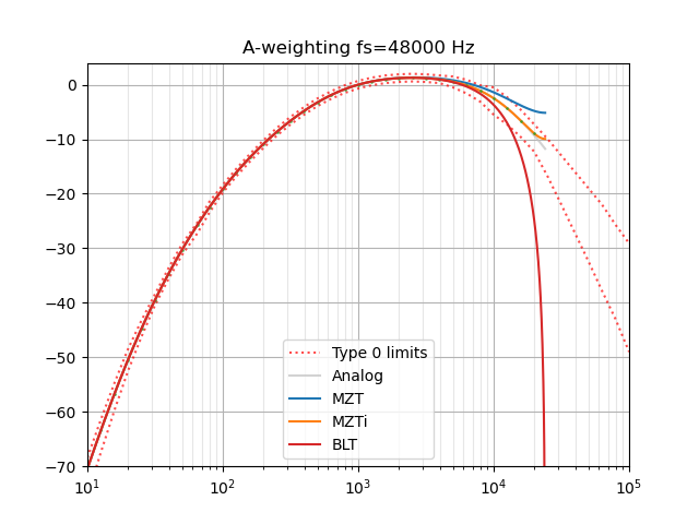
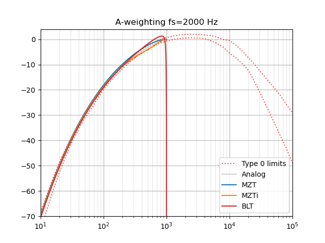
Note that this uses a bilinear transform and so is not accurate at high frequencies.
Apply an A-weighting filter to a sound stored as a NumPy array.
Use Audiolab or other module to import .wav or .flac files, for example. http://www.ar.media.kyoto-u.ac.jp/members/david/softwares/audiolab/
Translated from MATLAB script (BSD license) at: http://www.mathworks.com/matlabcentral/fileexchange/69


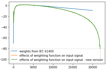
OK I should have mentioned first that my input signal is sampled at 44 kHz,
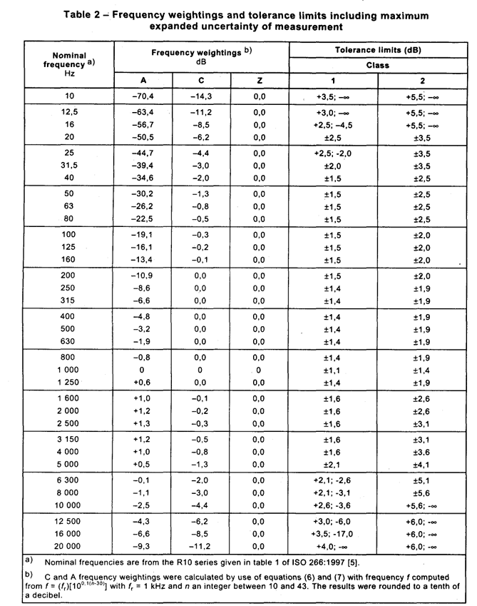
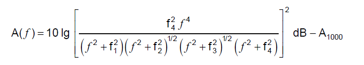
The "weights from IEC 61400" curve is just the plotting of the norm's formula:
i.e. the difference in dB between between an A_weighted spectrum and the same spectrum without weighting
So when I apply the A_weighting function over my white-noise signal, I get a filtered signal in return. I would expect that when I plot its spectrum minus the original spectrum ("effects of weighting function" plot), I would get the same response as the "weights from IEC 61400", at least until 20 kHz (fs/2).
The "polynom" curve was the plotting of NUMs/DENs from this first code's version, applied to the frequencies array and 10-logged:
poly = 10*np.log10(np.polyval(NUMs,f_norm)/np.polyval(DENs,f_norm))
but forget it, I have to dig on filtering's theory (I'm not a spectialist), plotting that and expecting it to be similar to "weights from IEC 61400" might not be relevant...
I've just tested your newer version, the results are indeed equal to this one's.