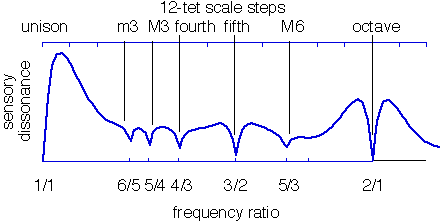
|
""" |
|
Python translation of http://sethares.engr.wisc.edu/comprog.html |
|
""" |
|
import numpy as np |
|
|
|
|
|
def dissmeasure(fvec, amp, model='min'): |
|
""" |
|
Given a list of partials in fvec, with amplitudes in amp, this routine |
|
calculates the dissonance by summing the roughness of every sine pair |
|
based on a model of Plomp-Levelt's roughness curve. |
|
|
|
The older model (model='product') was based on the product of the two |
|
amplitudes, but the newer model (model='min') is based on the minimum |
|
of the two amplitudes, since this matches the beat frequency amplitude. |
|
""" |
|
# Sort by frequency |
|
sort_idx = np.argsort(fvec) |
|
am_sorted = np.asarray(amp)[sort_idx] |
|
fr_sorted = np.asarray(fvec)[sort_idx] |
|
|
|
# Used to stretch dissonance curve for different freqs: |
|
Dstar = 0.24 # Point of maximum dissonance |
|
S1 = 0.0207 |
|
S2 = 18.96 |
|
|
|
C1 = 5 |
|
C2 = -5 |
|
|
|
# Plomp-Levelt roughness curve: |
|
A1 = -3.51 |
|
A2 = -5.75 |
|
|
|
# Generate all combinations of frequency components |
|
idx = np.transpose(np.triu_indices(len(fr_sorted), 1)) |
|
fr_pairs = fr_sorted[idx] |
|
am_pairs = am_sorted[idx] |
|
|
|
Fmin = fr_pairs[:, 0] |
|
S = Dstar / (S1 * Fmin + S2) |
|
Fdif = fr_pairs[:, 1] - fr_pairs[:, 0] |
|
|
|
if model == 'min': |
|
a = np.amin(am_pairs, axis=1) |
|
elif model == 'product': |
|
a = np.prod(am_pairs, axis=1) # Older model |
|
else: |
|
raise ValueError('model should be "min" or "product"') |
|
SFdif = S * Fdif |
|
D = np.sum(a * (C1 * np.exp(A1 * SFdif) + C2 * np.exp(A2 * SFdif))) |
|
|
|
return D |
|
|
|
|
|
if __name__ == '__main__': |
|
from numpy import array, linspace, empty, concatenate |
|
import matplotlib.pyplot as plt |
|
|
|
""" |
|
Reproduce Sethares Figure 3 |
|
http://sethares.engr.wisc.edu/consemi.html#anchor15619672 |
|
""" |
|
freq = 500 * array([1, 2, 3, 4, 5, 6]) |
|
amp = 0.88**array([0, 1, 2, 3, 4, 5]) |
|
r_low = 1 |
|
alpharange = 2.3 |
|
method = 'product' |
|
|
|
# # Davide Verotta Figure 4 example |
|
# freq = 261.63 * array([1, 2, 3, 4, 5, 6]) |
|
# amp = 1 / array([1, 2, 3, 4, 5, 6]) |
|
# r_low = 1 |
|
# alpharange = 2.0 |
|
# method = 'product' |
|
|
|
n = 3000 |
|
diss = empty(n) |
|
a = concatenate((amp, amp)) |
|
for i, alpha in enumerate(linspace(r_low, alpharange, n)): |
|
f = concatenate((freq, alpha*freq)) |
|
d = dissmeasure(f, a, method) |
|
diss[i] = d |
|
|
|
plt.figure(figsize=(7, 3)) |
|
plt.plot(linspace(r_low, alpharange, len(diss)), diss) |
|
plt.xscale('log') |
|
plt.xlim(r_low, alpharange) |
|
|
|
plt.xlabel('frequency ratio') |
|
plt.ylabel('sensory dissonance') |
|
|
|
intervals = [(1, 1), (6, 5), (5, 4), (4, 3), (3, 2), (5, 3), (2, 1)] |
|
|
|
for n, d in intervals: |
|
plt.axvline(n/d, color='silver') |
|
|
|
plt.yticks([]) |
|
plt.minorticks_off() |
|
plt.xticks([n/d for n, d in intervals], |
|
['{}/{}'.format(n, d) for n, d in intervals]) |
|
plt.tight_layout() |
|
plt.show() |


Hmmm.
https://gist.github.com/jpivarski/5e4908b09f4f9a244496d4d214e5c769/raw/c43bfaec1927400f0ec39acf0f592ca82d2927ff/hydrogen-scale-2.wav
That's all from me. (Making the tone less realistic by focusing on only one kind of transition didn't make it any less warbly. There are doublets/nearly equal frequencies in every transition; it has to do with having so many energy levels that are nearly equal to each other.)