Skip to content

Instantly share code, notes, and snippets.

@endolith
Last active September 14, 2024 01:28
Show Gist options
  • Save endolith/148112 to your computer and use it in GitHub Desktop.
Save endolith/148112 to your computer and use it in GitHub Desktop.
A-weighting audio files in Python
#!/usr/bin/env python
# -*- coding: utf-8 -*-
"""
Translated from a MATLAB script (which also includes C-weighting, octave
and one-third-octave digital filters).
Author: Christophe Couvreur, Faculte Polytechnique de Mons (Belgium)
couvreur@thor.fpms.ac.be
Last modification: Aug. 20, 1997, 10:00am.
BSD license
http://www.mathworks.com/matlabcentral/fileexchange/69
Translated from adsgn.m to Python 2009-07-14 endolith@gmail.com
"""
from numpy import pi, polymul
from scipy.signal import bilinear
def A_weighting(fs):
"""Design of an A-weighting filter.
b, a = A_weighting(fs) designs a digital A-weighting filter for
sampling frequency `fs`. Usage: y = scipy.signal.lfilter(b, a, x).
Warning: `fs` should normally be higher than 20 kHz. For example,
fs = 48000 yields a class 1-compliant filter.
References:
[1] IEC/CD 1672: Electroacoustics-Sound Level Meters, Nov. 1996.
"""
# Definition of analog A-weighting filter according to IEC/CD 1672.
f1 = 20.598997
f2 = 107.65265
f3 = 737.86223
f4 = 12194.217
A1000 = 1.9997
NUMs = [(2*pi * f4)**2 * (10**(A1000/20)), 0, 0, 0, 0]
DENs = polymul([1, 4*pi * f4, (2*pi * f4)**2],
[1, 4*pi * f1, (2*pi * f1)**2])
DENs = polymul(polymul(DENs, [1, 2*pi * f3]),
[1, 2*pi * f2])
# Use the bilinear transformation to get the digital filter.
# (Octave, MATLAB, and PyLab disagree about Fs vs 1/Fs)
return bilinear(NUMs, DENs, fs)
import sys
from scipy.signal import lfilter
import numpy as np
from A_weighting import A_weighting
try:
import soundfile as sf
except ImportError:
from scikits.audiolab import wavread
# (scipy.io.wavfile can't read 24-bit WAV)
def rms_flat(a): # from matplotlib.mlab
"""
Return the root mean square of all the elements of *a*, flattened out.
"""
return np.sqrt(np.mean(np.absolute(a)**2))
if len(sys.argv) == 2:
filename = sys.argv[1]
else:
filename = 'noise.wav'
try:
x, fs = sf.read(filename)
except NameError:
x, fs, bits = wavread(filename)
print(filename)
print('Original: {:+.2f} dB'.format(20*np.log10(rms_flat(x))))
b, a = A_weighting(fs)
y = lfilter(b, a, x)
print('A-weighted: {:+.2f} dB'.format(20*np.log10(rms_flat(y))))
@Yan-Iron
Copy link

Yan-Iron commented Aug 2, 2018

Dear all, I am new to digital signal processing. I am wondering, in order to get A weighted sound pressure level, should I first apply this function to the wav data read by functions like "scipy.io.wavfile.read" then convert it to SPL, or first convert wav data to sound pressure level then use this function for A weighting? Thanks in advance!

@endolith
Copy link
Author

endolith commented Aug 2, 2018

@shangyan0517 I would recommend:

  1. Using this version instead
  2. Use PySoundFile instead of scipy.io.wavfile.read

Then you need to figure out what your dBSPL ↔ dBFS conversion factor is. Depends on sensitivity of microphone, gain of preamp, etc.

It doesn't matter if you do SPL conversion first, then A-weighting, or A-weighting, then SPL conversion. Both are LTI operations.

@Yan-Iron
Copy link

Yan-Iron commented Aug 3, 2018

@endolith Thank you so much!

@masahf
Copy link

masahf commented Aug 21, 2020

@endolith Thank you for the helpful code.
I am new to digital signal processing.
I'm doing a project with digital MEMS microphones and using audiobusio library that has PDMin for recording over i2s with CircuitPython. My goal is to convert the digital output signal into dB SPL but still don't know how to do it :( Can I use this function for the I2S output signal?

@annezhangxue
Copy link

@endolith, Thank you for the code, it works out perfectly!
I am also new in acoustics, could you please let me know if this is based on octave band or one third octave band please?

Thanks.

@endolith
Copy link
Author

@annezhangxue It is not based on octave bands. 🤔 It's an IIR filter

@ThomQu
Copy link

ThomQu commented Oct 8, 2021

@endolith

Hi!

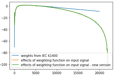
I've been testing your code and Idon't fully get it: It doesn't weight the signal at high frequencies. here's a fig with:

  • the A-weights from IEC 1672 norm (blue);
  • the polynom NUMs/DENs from your function (green);
  • the difference between the spectrum of an A-weigted white noise signal, and the same signal without A weighting.

As you can see, the polynom tends to zero for high frequencies, causing the curve 3 to diverge from the expected result...
image

I've buid up a polynom that gives exactly the same response as the norm coefficients (note the minus sign on A1000), but still, when i convert it to an analog filter with bilinear, the output is irrelevant :

    f1 = 20.598997
    f2 = 107.65265
    f3 = 737.86223
    f4 = 12194.217
    A1000 = -2.0
    
    NUMs = [(f4 ** 2), 0, 0, 0, 0]
    NUMs = np.polymul(NUMs, NUMs)
    DENs = np.polymul([1, 0 , 2 * (f1 ** 2), 0, f1 **4] , [1, 0, f2 ** 2])
    DENs = np.polymul(np.polymul(DENs, [1, 0, f3 ** 2]), [1, 0 , 2 * (f4 ** 2), 0, f4 **4])
    DENs = DENs * (10**(A1000/10))

Any idea to confirm / correct this?

BR

@endolith
Copy link
Author

endolith commented Oct 8, 2021

@ThomQu

  1. This version is only accurate at high sampling rates, because it's bilinear transformed from the analog filter.
  2. You shouldn't use this version anymore, as it says in the readme. The version mentioned in the readme is better at lower sample rates. (Edit: Actually I guess it's not yet. I have a better version with MZTi correction that I haven't pushed yet. I thought I pushed it a long time ago.)
  3. I don't understand your graph. Is it linear frequency axis or log?

@ThomQu
Copy link

ThomQu commented Oct 8, 2021

@endolith

That was quick, thanks!

  1. OK for that, but since the frequency-polynom doesn't match with the norm before building-up the filter, it looks that the final error is due to the polynom formula rather than the filtering process, am I right?
  2. OK I'm gonna try that other version right away
  3. Linear frequencies. Sorry my previous pic was crap, here's the full graph:
    image

@endolith
Copy link
Author

endolith commented Oct 8, 2021

@ThomQu

  1. I'm not sure I understand what you're doing. In this version, ABC_weighting() produces analog filter coefficients. Then A_weighting() converts it to a digital filter using bilinear transform (which has the discrepancy of going to zero at fs/2, so it's only accurate for low frequencies or if your sampling rate is high), then A_weight() actually applies that digital filter to a signal.
  2. Did you see my edit? The other version isn't actually going to be better at high frequencies, that was a mistake. I need to upload my improved version.
  3. So "weights from IEC 61400" is analog frequency response? And "effects of weighting function" is from processing digital white noise? That looks about as I would expect, since the digital filter drops to zero at fs/2. The discrepancy is due to bilinear transform. I don't understand what "polynom" is?

@ThomQu
Copy link

ThomQu commented Oct 8, 2021

OK I should have mentioned first that my input signal is sampled at 44 kHz,

The "weights from IEC 61400" curve is just the plotting of the norm's formula:
image
i.e. the difference in dB between between an A_weighted spectrum and the same spectrum without weighting

So when I apply the A_weighting function over my white-noise signal, I get a filtered signal in return. I would expect that when I plot its spectrum minus the original spectrum ("effects of weighting function" plot), I would get the same response as the "weights from IEC 61400", at least until 20 kHz (fs/2).

The "polynom" curve was the plotting of NUMs/DENs from this first code's version, applied to the frequencies array and 10-logged:

poly = 10*np.log10(np.polyval(NUMs,f_norm)/np.polyval(DENs,f_norm))
but forget it, I have to dig on filtering's theory (I'm not a spectialist), plotting that and expecting it to be similar to "weights from IEC 61400" might not be relevant...

I've just tested your newer version, the results are indeed equal to this one's.
image

@endolith
Copy link
Author

endolith commented Oct 8, 2021

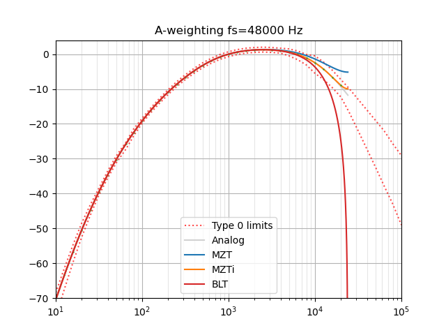
So I'm looking at my "improved" version from 2018, which is based on the MZTi method and it does indeed have better frequency response at high frequencies:

MZT vs MZTi vs BLT

But I think the reason I didn't push it was because I wasn't sure I was doing it right. "Since the mapping wraps the s-plane's jω axis around the z-plane's unit circle repeatedly, any zeros (or poles) greater than the Nyquist frequency will be mapped to an aliased location." And I'm not sure if those need to be removed first, depending on the sampling rate, etc. At lower sample rates it gets worse, so it still needs some work. (Also the aliased Nyquist tail could be pushed down a bit to improve the overall average accuracy.)

This paper just describes the same BLT solution as this gist, and has a table of the minimum required sample rate to meet the tolerances:

  A-weighting C-weighting
IEC 61672-1 Class 1 35 kHz 35 kHz
IEC 61672-1 Class 2 20 kHz 20 kHz
ANSI S.1-43 Type 0 71 kHz 72 kHz
ANSI S.1-43 Type 1 35 kHz 35 kHz
ANSI S.1-43 Type 2 20 kHz 20 kHz

There are probably other papers that describe better methods, I should look for them.

@endolith
Copy link
Author

@ThomQu @annezhangxue @shangyan0517 @frgos2 @masahf @mankind-nil @Zeokat

Can you all tell me how you use this code so I can improve it? I tried to fold it into a library with other related functions like THD+N calculators, etc. But people still comment on this gist, so maybe it's better for it to be self-contained? I assume you are all using the digital filter version and not the analog filter coefficients?

@ThomQu
Copy link

ThomQu commented Oct 11, 2021

@endolith

Personnaly, I am trying to build-up a library that wraps up a few key functions for quick audio files analyses. I've picked stuff from librosa, scipy, etc and got your code from some colleague's scripts. That's the reason why I went for that first version.

Thks for the info about the MZTi method, I'll look for a little help around to check what I can do with it.

Regards

@endolith
Copy link
Author

@ThomQu

Ok, so maybe I should just make an installable weighting filter library that does nothing else, and then you could use it in yours, etc? I tried combining it with other things like frequency estimation and THD calculation, but maybe those are too unrelated to combine.

@endolith
Copy link
Author

endolith commented Oct 15, 2021

I was asked on Stack Exchange for my MZTi code, even if crude, so here it is.

I don't think it's correct at very low sample rates, because of aliasing, but should be better at the typical 44.1 or 48 kHz. It's definitely wrong below fs = 2.5 kHz. In between, I think the MZTi zeroes are forcing it into compliance despite being poorly-transformed.

I don't think it makes much practical difference in dB levels vs the BLT method, by the way.

# Poles and zeros for analog filter from specification
z, p, k = ABC_weighting('A')

# Matched Z Transform:
T = 1/fs
z_MZT = np.exp(z*T)  # 4
p_MZT = np.exp(p*T)  # 6

k_MZT = k * ((np.prod(2*pi*1000 - z)/
              np.prod(2*pi*1000 - p)) *
             (np.prod(1 - exp(p*T - 2*pi*1000*T)))/
              np.prod(1 - exp(z*T - 2*pi*1000*T)))

# Tweak gain to actual magnitude response TODO: Why is this necessary?
w_MZT, h_MZT = signal.freqz_zpk(z_MZT, p_MZT, k_MZT, [1000/(fs/2)*pi])
k_MZT /= abs(h_MZT)


w = np.array([pi/3, 2*pi/3])
H = abs(signal.freqs_zpk(z, p, k, w*fs)[1] /
        signal.freqz_zpk(z_MZT, p_MZT, k_MZT, w)[1])  # relative magnitude error

# MZTi method of 0, 1/3, 2/3 Nyquist will not work, since response at 0 is 0.
H = np.concatenate(([1], H))

b1 = 0.5 * (H[0] - sqrt(H[0]**2 - 2*H[1]**2 + 2*H[2]**2))
b2 = (3 * (H[0] - b1) -
      sqrt(-3*H[0]**2 + 12*H[1]**2 - 6*H[0]*b1 - 3*b1**2 + 0j)
      ) / 6
b0 = H[0] - b1 - b2
b = np.array([b0, b1, b2])

z_correct = np.roots(b)

# TODO: Is this right?
z_MZTi = np.concatenate((z_MZT, z_correct))
p_MZTi = p_MZT
k_MZTi = k_MZT

# Tweak gain to actual magnitude response again TODO: Why?
w_MZTi, h_MZTi = signal.freqz_zpk(z_MZTi, p_MZTi, k_MZTi, [1000/(fs/2)*pi])
k_MZTi /= abs(h_MZTi)

And the reference is https://www.khabdha.org/wp-content/uploads/2008/03/optimizing-the-magnitude-response-of-mzt-filters-mzti-2007.pdf

@endolith
Copy link
Author

so maybe I should just make an installable weighting filter library that does nothing else

and maybe include bilinear as an option so people can compare with the results of other software?

@endolith
Copy link
Author

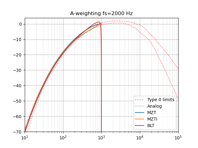
FYI, the MZTi version is accurate down to about 2.5 kHz:

redo 8 kHz
redo 8 kHz closeup

redo 3 kHz
redo 3 kHz closeup

redo 2 kHz
redo 2 kHz closeup

@rickou
Copy link

rickou commented Aug 9, 2023

@endolith your graph are very interresting !
how do you graph the type 0 limits ?

@rickou
Copy link

rickou commented Aug 10, 2023

Thank you endolith !

i just found the table from standard, and i'm little bit surprised because the values are not exactly the same.
image

do you still have the original table ? (i do not have the standard at my side, so i use google to find parts of it 🙃)
thank a lot !

@rickou
Copy link

rickou commented Aug 10, 2023

@endolith one more question about MZTi, have you push this improvement somewhere ? (i haven't found it ...)
My goal is to use the resulting coefficient in a microcontroller based hardware with IIR/FIR filtering functions, do you know if MZTi coefficient usable in those cases ? (i'm beginner in signal processing)
thank you !

@endolith
Copy link
Author

@rickou The values I used are from https://law.resource.org/pub/us/cfr/ibr/002/ansi.s1.4.1983.pdf

I think I only posted the MZTi code above https://gist.github.com/endolith/148112?permalink_comment_id=3928477#gistcomment-3928477

and again I have qualms about it, I'm not sure if it's handling the high-frequency poles/zeros correctly.

@rickou
Copy link

rickou commented Aug 11, 2023

Thank you ! now i understand the differences..

About the MZTi, i already read your post, do you have any clues that could explain why the high frequency poles/zeros could not be good ?
What can be wrong on signal or on response ?
Have you made some test with real waveforms ?

@endolith
Copy link
Author

do you have any clues that could explain why the high frequency poles/zeros could not be good ?

MZT appeals to me for high sample rates because the A-weighting filter is defined by precise pole locations, so it feels right to transform them this way and get a similar response. The problem is that when the sampling rate is too low, they are outside the Nyquist range and it introduces error. The i stage will then correct for this as much as possible, so it's still accurate down to 2.5 kHz, but it just feels kind of wrong to me to produce the wrong response and then patch over it with this bandaid.

@rickou
Copy link

rickou commented Sep 14, 2023

hum.. i think i understand.. to be honest i'm not so comfortable with digital filtering.
i have implemented this filter in embedded software and i will made some tests in next weeks in real situation comparing my implementation and sonometer.
but my preliminary tests on bench shows nothing bad. (i'm using 20k sample rate)

Sign up for free to join this conversation on GitHub. Already have an account? Sign in to comment